
 I have not kept it secret that I’m a fan of solar power. Leaving storage hangups aside for now, the fact that the scale of available power is comfortably gigantic, that perfectly efficient technology exists, that it’s hard-over on the reality axis (vs. fantasy: it’s producing electricity on my roof right now), and that it works well almost everywhere—what’s not to like? Did you trip over that last part? Many do. In this post, we’ll look at just how much solar yield one may expect as a function of location within the U.S.
The ancient Mayans laboriously accumulated a substantial set of observational data on solar illumination across America well ahead of the present need. Okay, it wasn’t actually the ancient Mayans. It was the National Renewable Energy Lab (NREL), who embarked on a 30-year campaign beginning in 1961, covering 239 locations across the U.S. and associated territories. Imagine this. How many people were even cognizant of solar power in 1961? Yet the forward-thinking scientists at NREL appreciated the value of a solid baseline dataset way back then. This level of foresight seems akin to the Mayans constructing a calendar going all the way to 2012. That’s all I’m saying. It’s a gift from the past.
I have often consulted and enjoyed the product of this work over the years—called the NREL Redbook, or more formally, the Solar Radiation Data Manual for Flat Plate and Concentrating Collectors. But with a snazzy blog post as motivation, I have taken it up a notch and produced a variety of graphical representations of the dataset to explore what it can tell us. Let’s begin the guided tour.
What’s in the Dataset?
In 1961, various sensors were installed in 56 locations distributed throughout the U.S. to measure solar illumination on an hourly basis. Measuring both diffuse and direct sunlight, it is possible to reconstruct what a flat panel (or concentrating collector) will receive in a particular orientation. In addition to the 56 “primary” stations, 183 “secondary” locations contributed meteorological measurements—including cloud cover—which were bootstrapped into the dataset by modeling the solar illumination. The map below illustrates the locations of the stations, leaving out the two stations in Puerto Rico and Guam.
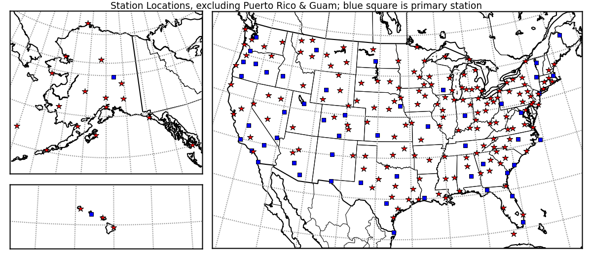
Primary (blue squares) and secondary (red stars) stations used in the NREL Redbook report.
A word about these maps before we go on. They are all equal-area projections (Albers), and each panel is scaled correctly relative to each other. Grid lines are at 5° intervals. All are generated via Python using matplitlib and Basemap. They are each 1200 pixels across, and may benefit from clicking to view full-size.
The original hourly data would be a bit unwieldy (though I do have an appetite for data, and may someday track down the full dataset). So instead, the Redbook presents monthly averages of daily energy accumulation measured in kWh/m²/day.
Because the “standard sun” deposits 1000 W/m² under clear conditions, the kWh/m²/day metric conveniently maps to the equivalent number of full-sun hours one receives per day. For example, typical locations in the U.S. average about 5 kWh/m²/day over the year for a flat panel facing south and tilted to the site latitude. This means about five hours of full, direct sunlight is normal. Of course, the sun is up longer than five hours (in fact, the yearly average is 12 hours, anywhere on Earth, neglecting refraction effects near the horizon). But factor in geometry and clouds, and we get down to 5. By geometry, I mean that the sun is not always directly in front of the panel. When the sun is near the horizon, the illumination of the panel is oblique, so that the panel effectively is foreshortened and has a geometrically reduced cross section for capturing the sun’s rays. A tracking mount removes most or all geometrical considerations, leaving only clouds and atmospheric transparency as factors.
Back to the dataset, which presents monthly averages of daily yields, together with an annual average, for a variety of panel orientations and tracking possibilities. Because the study spanned three decades, it is also possible to report meaningful minima and maxima for each month in each panel configuration.
Below is a sample for St. Louis, MO. Why do I pick St. Louis? Because it is (or was until 2008) a political bellwether state for presidential elections? Because Missouri is the “Show Me” state, and the scientist in me resonates with this attitude? Because it’s the Gateway to the West, where the killer solar potential sits? Well, all these are fine reasons, but really it’s because when I sort the list of stations based on virtually any measure, St. Louis always turns up right there in the middle of the list, making it a happy median.
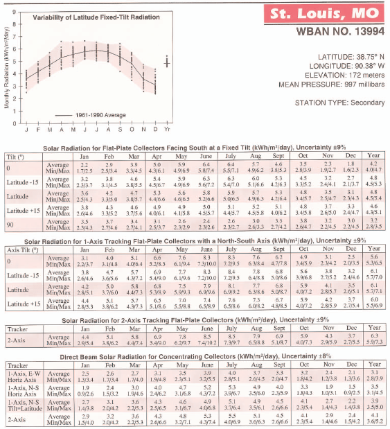
Available from the Redbook site.
Dissecting the page, location information and station type appear at upper right. At upper left, we see a plot of the annual pattern of illumination onto a flat panel oriented toward the south and tilted at the site latitude. A dot appears for every month in the 30-year campaign, and a pink slug indicates the full range of variability. On the right-hand side of this plot is a cluster of points indicating the yearly average yield.
Next are four blocks of numbers for:
- A fixed panel facing south, tilted to various degrees
- A panel tracking on a single north-south axis, either horizontal or tilted to various degrees
- A panel tracking the sun perfectly (2-axis)
- Concentration yield for various tracking schemes on one or two axes
I clipped out the final block of monthly climatic conditions in the image above.
For each block, the monthly averages and minima/maxima are presented, the annual average appearing at right. This page represents summary statistics, but monthly values spanning 360 months are also available.
What Can We Learn?
Using the St. Louis data as an example, what can we make of all these numbers?
Let’s say you buy a panel and want to know how to get the most from it. If you don’t want to mess with tracking, then according to the St. Louis data it hardly matters how you tilt the panel, so long as it’s within 15 degrees of site latitude: you’ll get an annual average of 4.6–4.8 full-sun-equivalent hours per day. But if you want more constancy throughout the year, the latitude-plus-15 solution is better. You’d sacrifice 4% on the annual average (4.6 vs. 4.8), but the variation throughout the year is from 72% to 113% of the average (3.3 to 5.2), whereas if we went for latitude-minus-15, we’d see 56% to 131% variation (2.7 to 6.3). Of course the variation in both cases is bigger if considering minima and maxima instead of the monthly averages over 30 years.
Tracking and Concentration
What about tracking? One-axis tracking (much simpler than dual-axis tracking) buys a 27% boost over a fixed panel (6.1 vs. 4.8). Is it easier and cheaper just to buy 27% more panels and avoid tracking complications? Often it will be. Going to a full-up 2-axis tracker buys only 3% over the 1-axis tracker (6.3 vs. 6.1). That’s because a 1-axis tracker with the rotation axis tilted at the latitude angle and facing north (thus parallel to the Earth’s axis of rotation) will never see the sun more than 23.5° away from the panel direction. The cosine projection of a 23.5° offset then results in capturing 92% of the light that a perfectly-pointed panel would see—and this is the worst-case projection, around the solstices. On average, the effect drops to something like a 4% loss, in rough agreement with the 3% number pulled out of the NREL data. One-axis tracking will generally see greater seasonal variation than the fixed-panel analog, due to much-improved performance in the summer.
If you want to do concentrated solar power, Missouri might not be the ideal place. At its best (2-axis tracking; and tracking is vital to concentration), we only get 85% as much as we would from a fixed panel (4.1 vs. 4.8). Of course, this compares area of the concentrator to area of the panel. If the concentrator is dirt-cheap compared to panels, it could turn out to be a better route. But tracking will always increase complications, cost, and maintenance issues. Concentration (and thus solar thermal) strongly favor the cloudless skies characteristic of desert locales.
Inferring Weather
Somewhat more interesting is to compare 2-axis tracking in the flat panel vs. concentration cases, since geometrical factors are removed and we are left with a sense of how much direct sun is available at a site. In St. Louis, the concentrator pulls in 65% of what the flat panel would (4.1 vs. 6.3). This says that 65% of the light hitting the tracking panel in St. Louis is from direct vs. indirect sunlight. When clouds are in the way, concentrators become virtually useless, while the flat panel still enjoys diffuse light from the bright cloudy sky. Because direct sun generally delivers more light than its diffuse counterpart, we can say that the skies over St. Louis are cloudy more than 35% of the time during daylight hours. On a monthly basis, we can ascertain that October is the month with clearest skies (69% of light from direct sun), while May is the cloudiest (62%). Not a great deal of variation, actually.
So that’s a snapshot of the type of information available in the NREL Redbook. Now let’s expand our scope beyond the midwest.
Comparing Sites
I copy below a table that appeared in an earlier post. The table represents the best location in the NREL database (Dagget, near Barstow, CA), St. Louis as a typical place, the worst place in the continental U.S. (on the Olympic Peninsula), and a few extras for flavor. For each location, three modes are considered: flat panel tilted at latitude (typical situation); flat panel with 2-axis tracking of the Sun; and concentration employing 2-axis tracking. For each mode and location, three daily-average numbers are given: worst average month—yearly average—best average month.
| Location | Fixed Tilt | 2-axis Tracking | Concentration |
| Dagget, CA | 5.2—6.6—7.4 | 6.8—9.4—12.0 | 5.4—7.5—9.7 |
| St. Louis, MO | 3.1—4.8—5.9 | 3.7—6.3—8.5 | 2.4—4.1—5.5 |
| Quillayute, WA | 1.5—3.4—4.8 | 1.7—4.4—6.8 | 1.0—2.6—4.0 |
| San Diego, CA | 4.6—5.7—6.5 | 5.9—7.4—8.9 | 4.5—5.3—6.3 |
| Fairbanks, AK | 0.3—3.3—5.6 | 0.3—4.7—8.7 | 0.3—2.9—5.3 |
The thing that’s always impressed me most about the NREL dataset is the fact that the worst location in the continental U.S. is only a factor of two worse than the best solar location. Intuitively, I would expect the Mojave Desert to outperform the Olympic Peninsula rain forest by leaps and bounds. But a meager factor of two! Even Fairbanks, Alaska performs well on the yearly average metric.
On to the Graphs
Enough with the tables of numbers. Let’s look at some graphical results.
Fixed Panel, South at Latitude
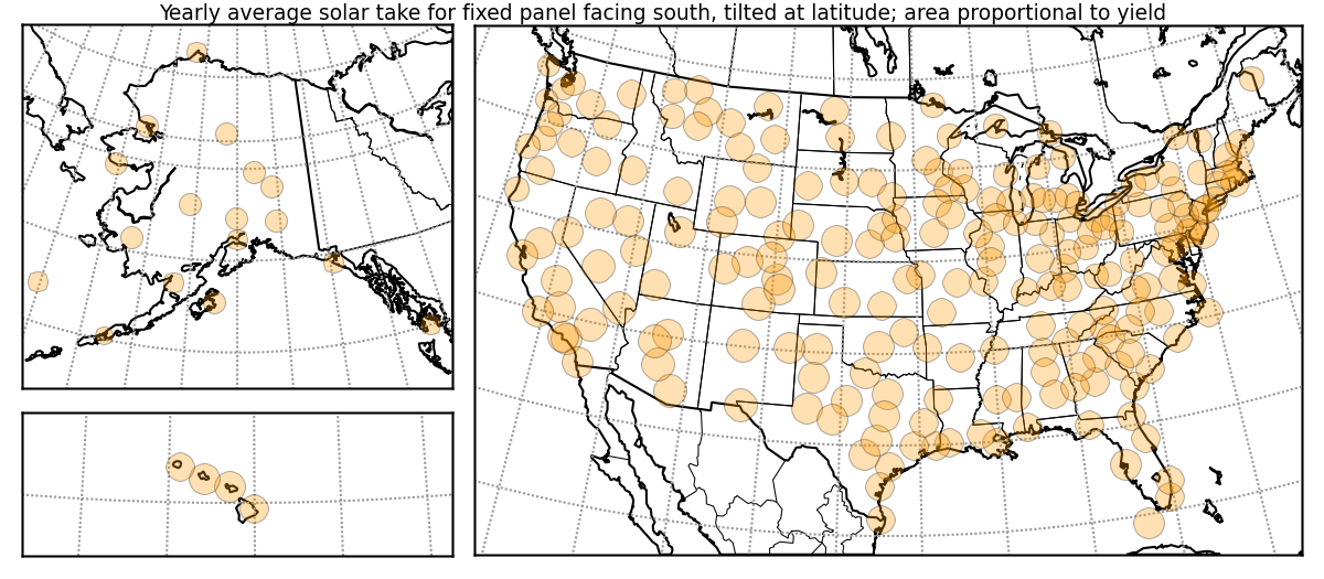 Above is a graphical representation of the yearly averages from each of the stations. The area of each circle corresponds to the solar yield, so at a glance we can compare relative performances across the country. If your brain works like mine does, the shocking thing is how similar all the circles are! Are they really different in size? At a glance, it’s hard to identify cruelly disadvantaged sites. On closer inspection, we can tell that the Pacific Northwest coast has smaller dots than the Desert Southwest. And the Alaskan spots are smaller than most (same map scale, so direct comparisons valid). But mostly I see a lot of suns out there, folks.
So my question to you is: Are you thinking right now that your location may be better for solar than you thought before reading this post?
Let’s invert the question to ask how large the solar array would have to be to deliver the same annual energy as a function of location.
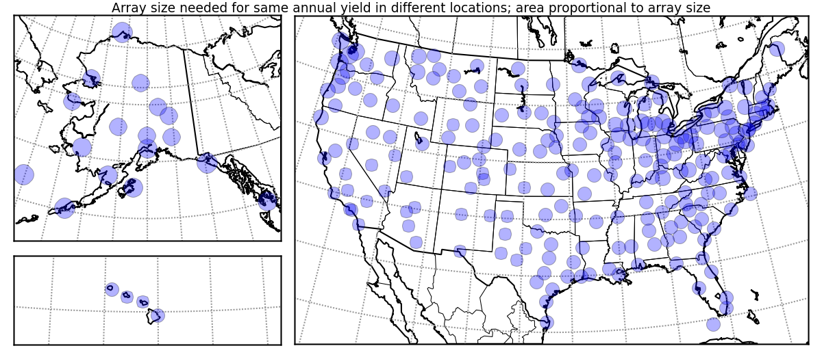 Same story from a different perspective: the array size (cost) does not look grossly different no matter where you go. Note that this is not the area of solar collectors needed for each area: those dots would generally be too small to see! Rather, it’s just the relative size in each location to deliver the same amount of annual energy.
Yearly Variation
Yearly averages are nice as a composite number, and is the most relevant metric for the ubiquitous grid-tie systems taking advantage of annualized net metering. But for stand-alone installations, unless your electricity use correlates with summer (as may be the case for air conditioning, refrigeration, or pumping water for irrigation), the system needs to be sized based on the poorest monthly performance rather than the annual average. If we had long-term storage (liquid fuels would be nice), we could ignore seasonal variations. Unfortunately, that’s not where we are—right now or in the foreseeable future.
So how does a fixed panel—pointing south and tilted to site latitude—perform across the year? I’ve got just the graphic for you.
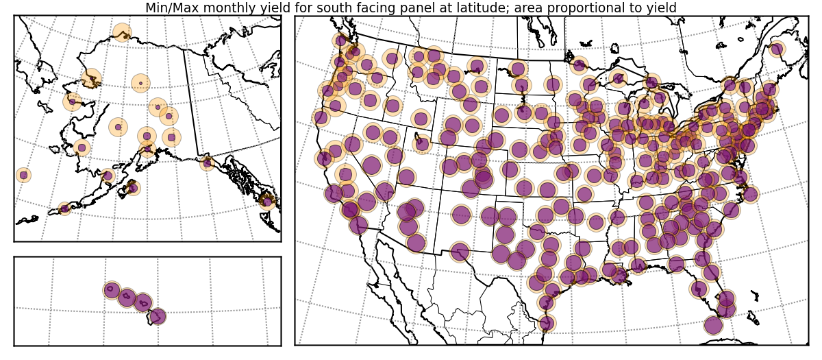 Now we have circle areas sized to reflect the maximum-yield month (can be different months for different sites) and the minimum-yield month (most commonly December). So what pops out? The Texas panhandle is remarkably steady year-round. Don’t try to hawk your giant battery banks there! Head to the Pacific Northwest coast for that, where the variation is far more pronounced. Latitude clearly plays a role in stomping on winter performance, but it’s not all there is to the story. Note that Montana and the Dakotas outperform the Great Lakes region in winter despite a higher latitude.
Alaska is a whole different story. Huge variations. Forget about reaping much sunlight in December near the Arctic Circle (nada at Barrow, the northernmost point in the sample). On the flip side, the long summer days make these locales comparable to many summer sites in the lower 48. And this even with a south-facing panel missing a lot of the fun when the rising and setting sun slip well to the north, behind the panel.
Solar Extremes
The fixed panel minimum/maximum is perhaps a very practical representation given the ease and predominance of this mounting option. But if we look instead at the two-axis (non-concentration) tracking, we get to ask how much the actual sunlight varies at a site. A fixed south-pointing panel misses substantial sunlight opportunities in the morning and evening around summer solstice, when the sun is north of the east-west line.
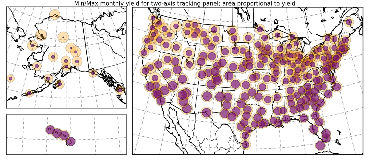
The winter-time performance is not substantially enhanced by tracking, especially for higher latitudes where a south-facing tilted panel is well situated to take in the whole show. But the summertime gain can be substantial. This has the effect of modestly enhancing aggregate yearly yield, but also results in larger variations throughout the year.
A Look at the Weather
We can play the same game we did for St. Louis in regard to evaluating direct vs. diffuse light by comparing the two-axis tracking results with and without concentration. Here I restrict attention to the months of December and June for all locations, and for each month form a ratio of concentration yield to flat panel yield (concentration is always less per square meter of collector vs. panel). I make an outer circle for June (sized the same for all locations) and an inner circle for December (also of uniform size). The grayscale indicates the degree of cloud opacity: darker is cloudier. For high-latitude stations in Alaska, I ignored points for which the daily average yield came out to 0.5 hours or less, opting instead to turn these winter interiors fittingly black.
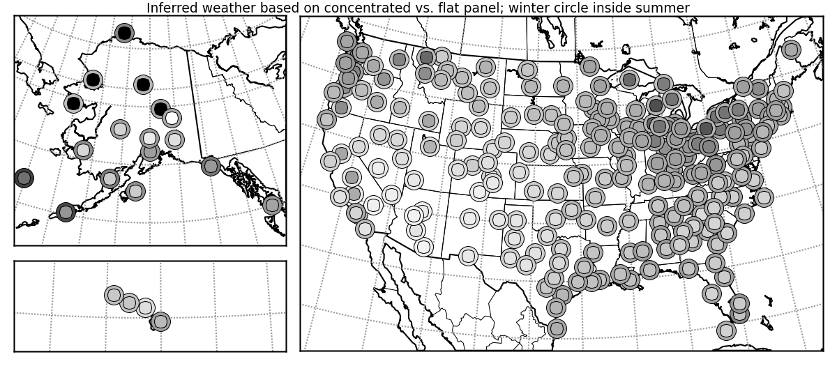 The view is interesting, I find. Dark on the outer annulus means a higher prevalence of clouds in the summer, while dark in the middle means cloudy winters. Seattle measures the same for both. Winters around the Great Lakes appear to be darker than those in Seattle (Erie, PA and Traverse City, MI are the standout dark ones). The Southeastern U.S. shows the signature of summer storms. San Diego and Los Angeles are sunnier in December than in June due to the “June Gloom” marine layer. Alaska tends to have cloudier summers than winters. Hawaii, as in most measures, is pretty constant year-round.
But as interesting as this plot might be, don’t let it be the deciding factor about whether a location is amenable to solar power. The previous maps are far better suited for that evaluation, addressing the solar potential directly. For instance, the statement above that it is sunnier in San Diego in December than in June does not translate into greater solar potential in December than June: the days are shorter and the sun at a lower elevation. It’s just that the fraction of daylight hours that the sun is directly visible is greater in the December than in June in San Diego.
Sizing for Variability
Thirty years of good data is a wonderful thing. The bad years and the good years are well represented. And three decades is a timescale commensurate with the likely lifetime of a photovoltaic (PV) installation.
In sizing a PV system, we could do the easy thing and base the size on the yearly average value for the appropriate panel orientation. But variability will mean underperformance in winter and overabundance in summer. On an annualized net-metering scheme for a grid-tie system, this is perfectly peachy, and one needs go no further.
As a case study to see if this whole NREL business is really a useful predictor, I can use performance measurements from a friend’s grid-tie system here in San Diego. The system has a nameplate capacity of 2592 W: 12 panels rated at 216 W each (based on 1000 W/m² input at 1.5 airmasses and 25 °C). The inverter efficiency and other minor losses put the AC rating at 2267 W (87.5% efficient). Over the last year, the system generated 4447 kWh, amounting to an average of 5.35 hours of full-sun-equivalent per day. The panels face south at a modest inclination of about 12°, so we would expect a performance somewhere between the average San Diego values of 5.0 hours for 0° (horizontal) orientation and 5.6 hours for latitude-minus-15° (17.8° tilt). Given year-to-year variations, we land close enough to the mark for me!
But what if you’re trying to satisfy a monthly net metering scheme, or—like me—you aim for off-grid performance using batteries and don’t have seasonal-timescale storage?
That’s where the monthly database comes in handy. For a given location and panel orientation, we can assess how often a month will come along dishing out a performance lower than some threshold. I like to frame said threshold as an “overbuild factor.” In other words, if the array is sized strictly according to the yearly average, one might expect it to underperform about half the time, so that we should scale up the system by some factor to cover the weaker periods. The greater the downward variation, the larger the overbuild factor must be.
For instance, let’s look at a panel tilted at site latitude for St. Louis. The yearly average is 4.8 full-sun equivalent (FSE) hours per day, but in December we only expect 3.1 FSE hours on average. So we could overbuild the nominal system by the factor 4.8/3.1 = 1.55×. Yet the worst December in the period from 1961–1990 resulted in only 2.3 FSE hours per day, so perhaps we should overbuild by 4.8/2.3 ˜ 2× to be “30-year safe.”
More usefully, we could turn the data into a frequency-based analysis via curves like the following.
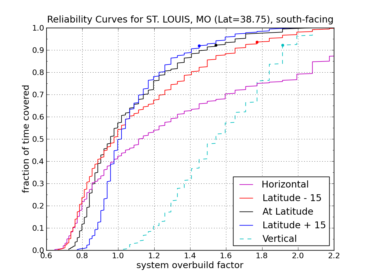
Indeed, for the black curve, representing a panel tilted to the site latitude in St. Louis, we see that in order to be 100% covered, we need a factor of 2 overbuild. But we can still get 95% coverage by lowering the system size to 1.7× or so: a 15% reduction in system size costs only 5% in reliability. 90% reliability needs only a 50% overbuild (1.5×).
Other curves are represented on the plot corresponding to different panel orientations, and all are referenced to the latitude-tilt yearly average. In other words, let’s say we decide we would need a 2.0 kW PV system tilted at latitude to satisfy our annual average energy need in St. Louis. If we then tighten the requirement to monthly performance and demand adequate solar resource 90% of the time, we would have to scale up the latitude-tilted system by a factor of 1.5 to 3.0 kW to meet our quota. But if we tilted the system to latitude-plus-15°, we can install a slightly smaller system (2.8 kW) and achieve the same effect. Other choices are not as favorable in this case, although by the time we get up to a 4.0 kW system (2× over-build), four of the five panel orientation choices are meeting the need.
Dots point out the reliability you’d get by using the worst monthly average (rather than minimum) for the panel orientation in question. For example, at latitude-plus-15 in St. Louis, the worst month gets 3.3 FSE hours, which compared to the tilt-at-latitude average of 4.8 suggests an overbuild of 1.45, which it turns out will provide adequate monthly energy 92% of the time.
The curves are “steppy” because the database values are rounded to one decimal place in kWh/m²/day (or FSE hours). The height of a step is an indication of how many months of the 360 months in the study produced that same performance.
Now let’s look at some other cases.
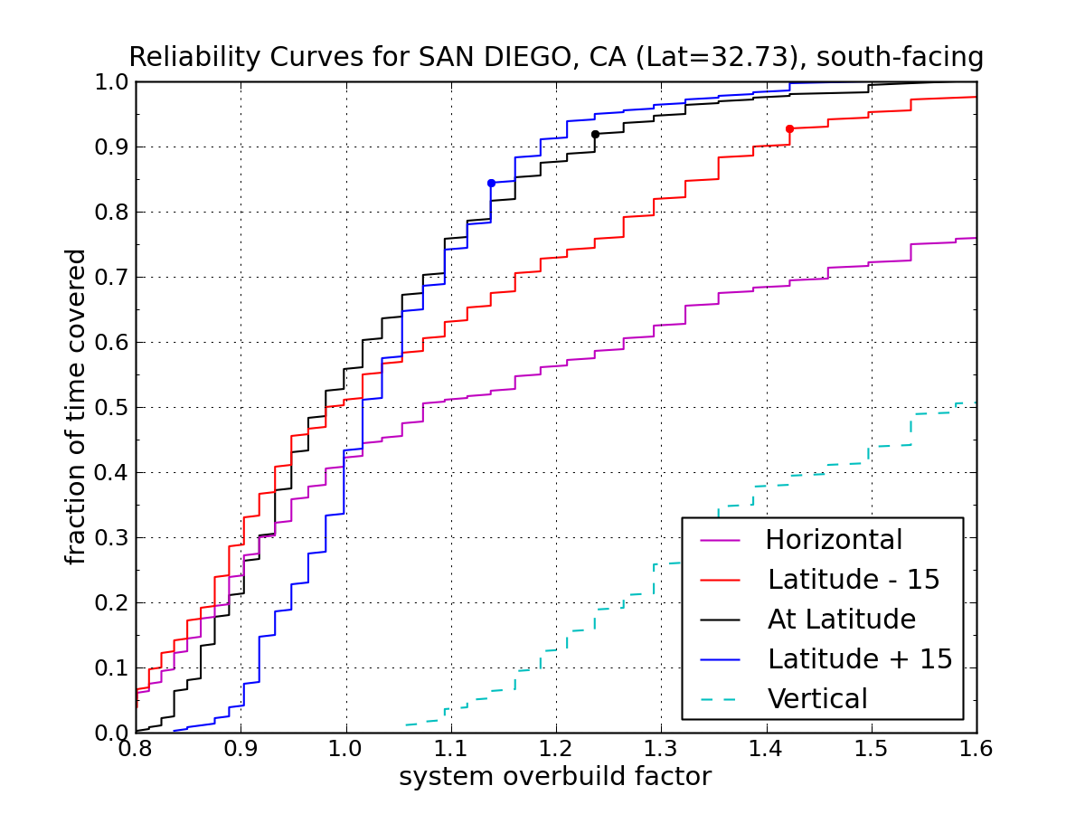
In San Diego, the near-constancy of weather means we can get 90% reliability with just a 20% over-build, or nearly full reliability with a 50% over-build—provided the panels are tilted at latitude or a little steeper. Vertical panels are not so useful.
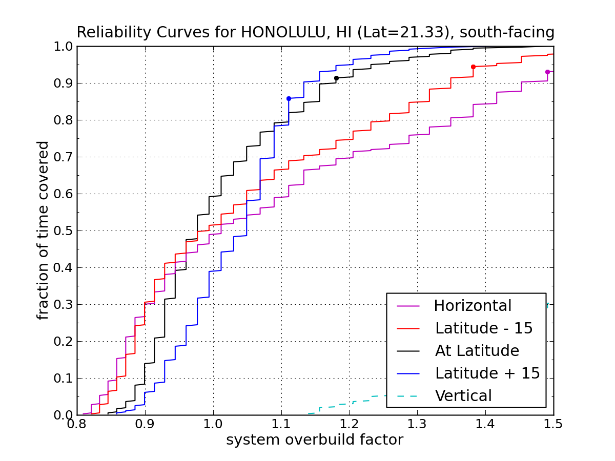
In a similar vein, the constant conditions of Honolulu tolerate even smaller overbuild factors for covering unusually bad months. At this latitude, a south-facing vertically-oriented panel is just plain stupid.
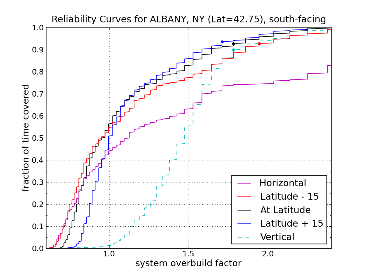
Let’s head to New York State, where we find slightly higher overbuild requirements than in St. Louis (plus, the baseline number of average sun-hours per day will be smaller). The latitude-plus-15° case again edges out the other choices, although all but the horizontal orientation converge by the time we exceed 90% reliability.
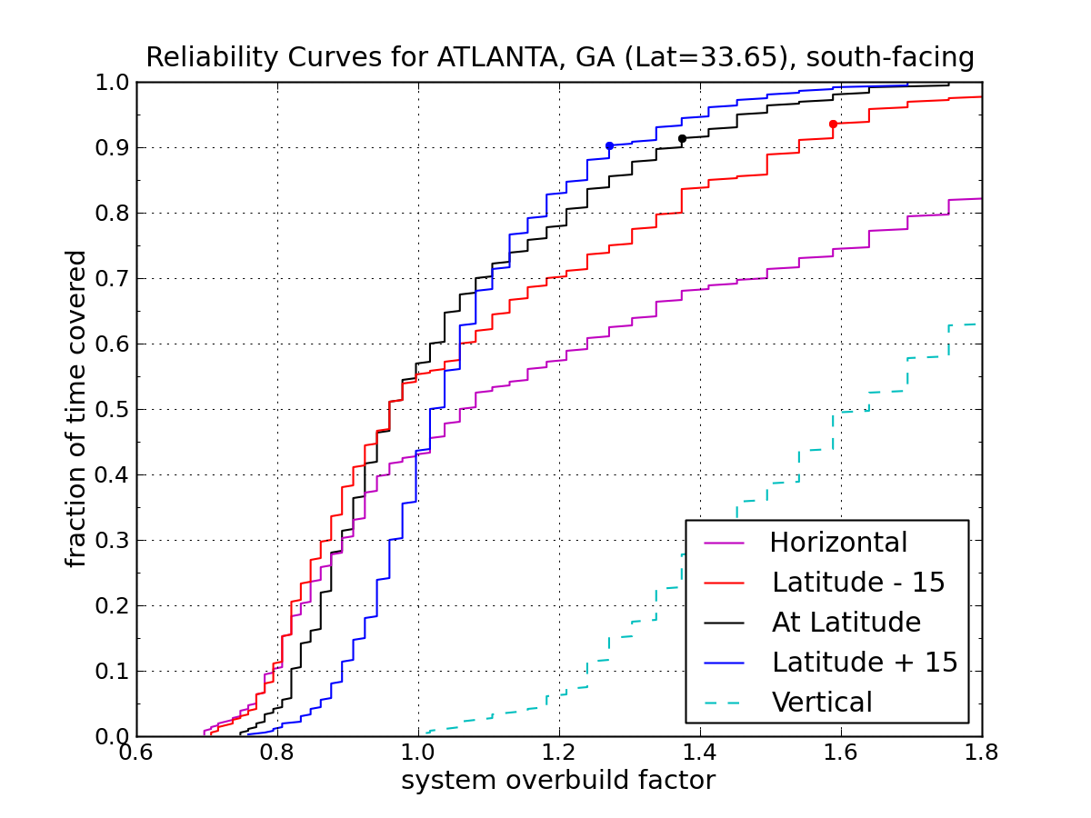
In Atlanta, a 50% overbuild puts you in good stead for latitude and latitude-plus-15° tilts.
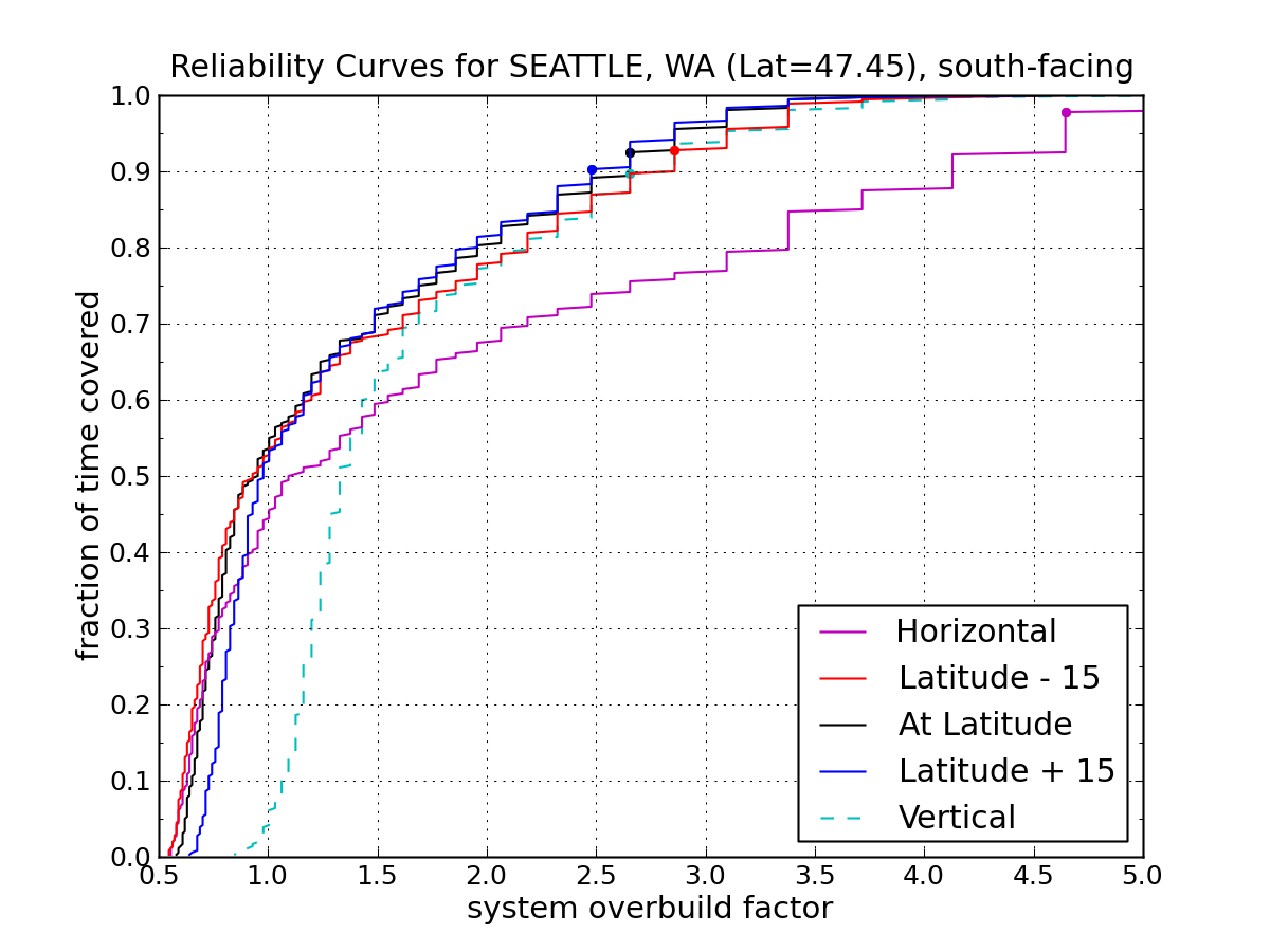
Seattle is an interesting case. The rising curves take their sweet time reaching the realm of reliability. But on the other hand, as long as you don’t lay the panel flat, it hardly matters what you do. In any case, we don’t hit reliable-land until a factor of 2.5–3 overbuild.
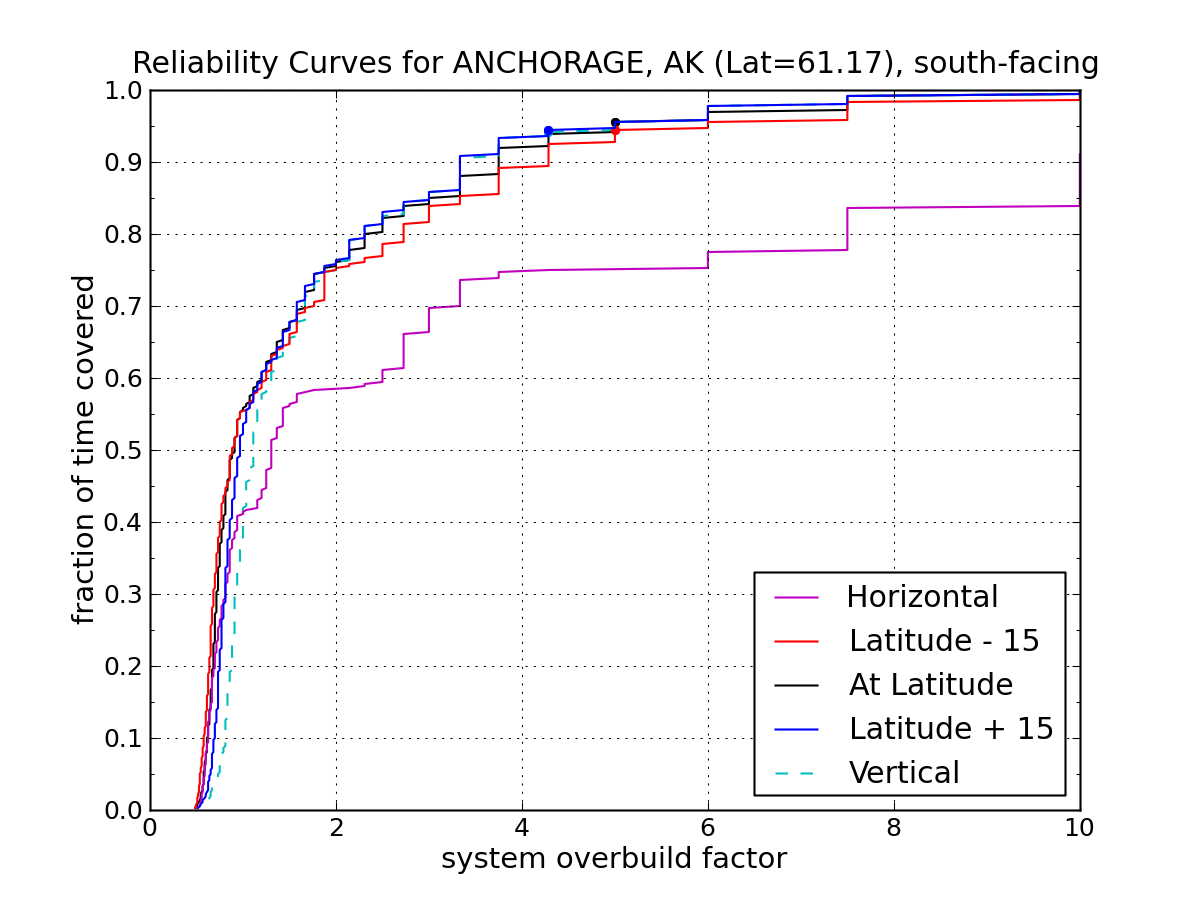
Anchorage, Alaska is a similar story—but more exaggerated. It hardly matters what orientation the panel is in, as long as it’s tilted up at least 45°. But you’ll need a 4× overbuild to cope with the worst of the winter months.
Note that in every one of the cases above, the latitude-plus-15° curves offered the lowest overbuild factor once into the range above 80% reliability. Over-tilting the panels pays off in the dismal parts of the year. Also, the dots based on the minimum reported month generally land in the 90–95% range.
All Together, Now
Seven down, 232 to go! Or why don’t I just put it into map form and hit everything with one swat?
Again using the annual average yield as the baseline, by what factor must we overbuild a system to get 90% or 95% coverage on a monthly basis? The map below shows the situation.
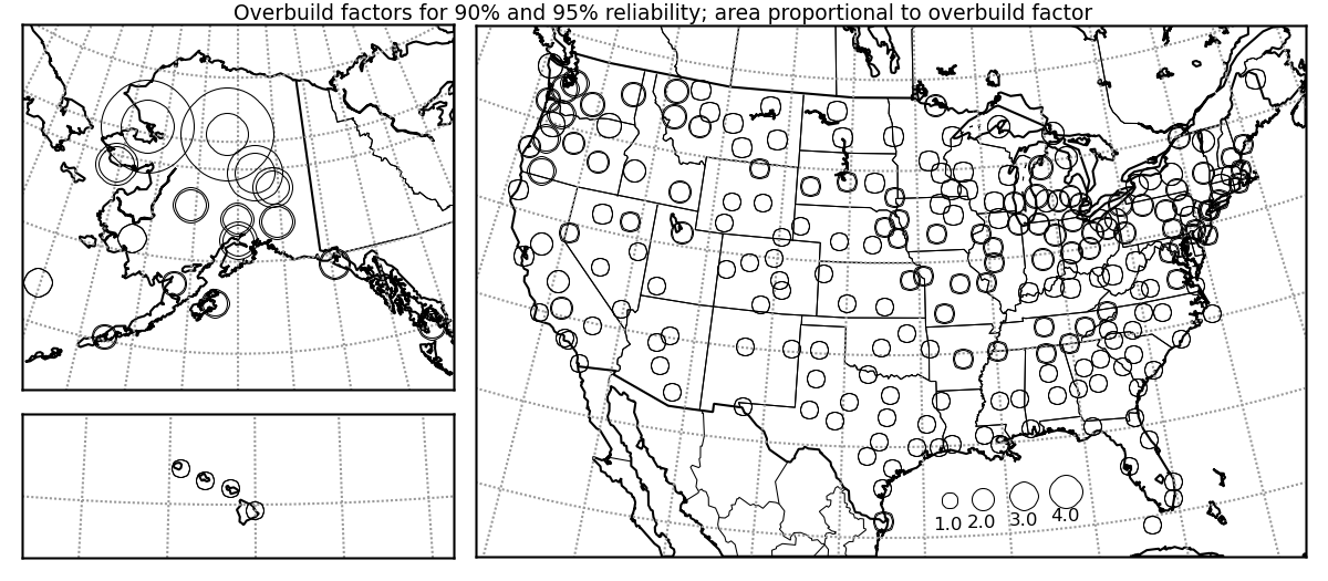 Less colorful than its cousins, each circle is area-scaled to represent an overbuild factor (legend appears in the Gulf of Mexico). For many sites, the two circles are indistinguishable. This suggests that 100% reliability is not far behind. But things go a little berserk in Alaska.
Let’s fold into this the differing annual yields as a function of location. What size array would you need to install to meet the same energy delivery requirement 90% and 95% of the time?
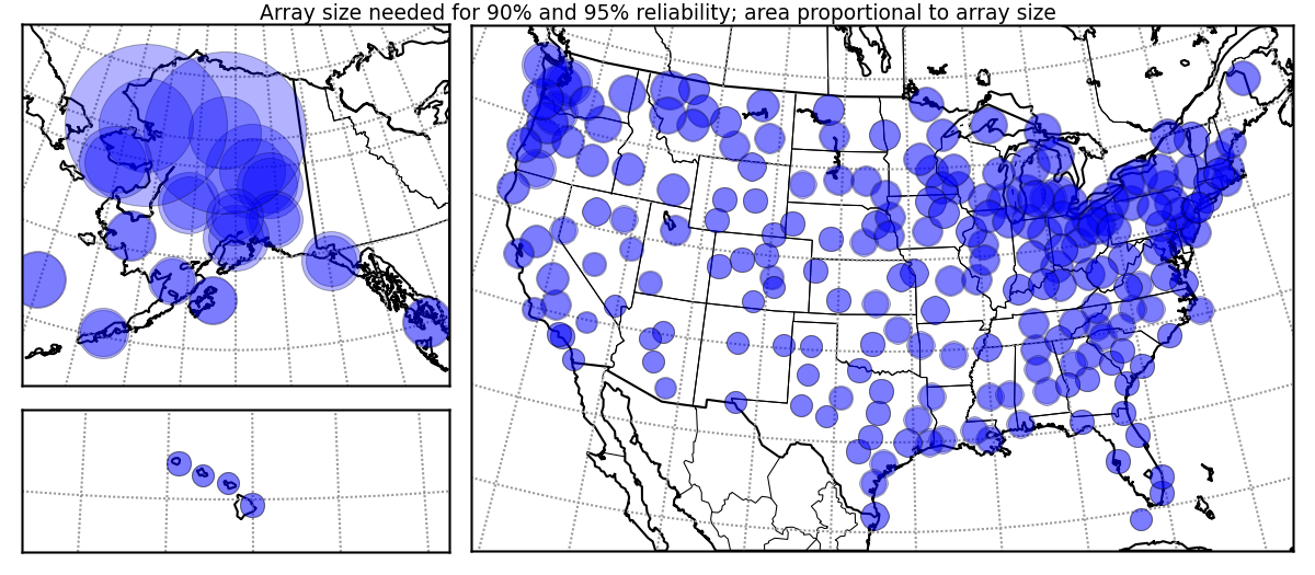 Again, the area of the circles scale with the size of the array needed. Now you see Alaskan winters taking their toll on year-round reliable performance. Too bad that off-grid is so Alaska—but at least northern Alaska isn’t having it.
Why Not 100% Reliability
Why did I stop short and satisfy myself with a mere 90–95% reliability? Well, the shallow slopes of the curves at the high end offer a hint. Filling in that last gap in reliability costs dearly in system size. My PV system at home keeps the batteries up to snuff about this fraction of the time. In dark times, I fall back on utility power. But what if I couldn’t do this?
It is a recent phenomenon that people live their lives not adapting to the whims of nature. Many of us run numerous aspects of our lives on a rigid schedule in disregard of the weather, the season, etc. We expect energy to be available 100% of the time and take it for granted. It was not always so, and it need not be true in the future. When energy runs a little short, it’s actually not that hard to modify behaviors to get through the crunch. Absolute rigidity and a 100% reliability requirement can push a stand-alone PV system into ridiculous proportions.
So relax. During a shortage, read a book by LED light rather than watching TV. Turn off the fridge (winter is the tough time, anyway) and store food outside or in a cooler garage. Cope. If only 5% of your time is spent in modified mode, how bad is this, really? The variety, challenge, and awareness of one’s resources can easily make it worthwhile. And a period of relative abundance is around the corner to make up for the shortfall. Just learn to ebb and flow, and you’ll feel more connected to the world as a result.