Revisiting the Shale Oil Hype: Technology versus Geology

The press has been all abuzz the past few weeks speculating on what the drop in oil prices will mean for U.S. shale oil (tight oil) production. Pundits have been falling over themselves quoting various estimates of the breakeven cost of production in this play or that, and rushing to be the first to declare a peak in the Bakken, Eagle Ford, Niobrara or wherever.  The Baker-Hughes rig count, which comes out every Friday, has become a must-read for people who probably had never heard of it a few months ago. Even the U.S. Energy Information Administration (EIA), based on estimates, suggests production is declining in three big shale oil plays.

The industry, on the other hand, has been more circumspect. They point to productivity gains being made in drilling and completion technology that lower costs, and suggest they are developing a backlog (aka “fracklog”) of wells that have been drilled but not completed, hanging in abeyance for the inevitable oil price rise (half or more of the cost of completing a well is the fracking). Keeping a stiff upper lip in the face of harsh pricing realities, many companies are telling investors that despite slashing capital expenditures on drilling and exploration (in some cases by more than 40%), production will be maintained and even rise. Others, such as Whiting, are putting themselves up for sale or, in the case of Quicksilver, declaring bankruptcy.

In my Drilling Deeper report published last October I stuck my neck out and made projections of future production by play based on drilling rates and well quality, not price, although price and drilling rates are closely linked. This was based on an analysis of all well production data by play which showed:

• Shale oil plays like the Bakken and Eagle Ford have field declines of 38-45% per year without new drilling. The Bakken requires some 1,700 new wells per year to maintain current production and the Eagle Ford about 2,800.
• Shale plays are not uniform in terms of reservoir quality and well productivity. Inevitably industry drills its best locations first. Geology will always trump technology in the long term and well quality will decline as plays mature.
• There are a finite number of places to drill, and although spacing wells too close together may increase short term production rates, it will not result in a higher recovery of the resource in the long term due to well interference. Well interference will not generally become evident until 12-24 months have elapsed, and is now indicated in top counties of the Bakken and Eagle Ford plays.

Given this, it is a no-brainer that production is going to fall if drilling rates decline as much as inferred from the 40+% fall in rig count since October. The “Most Likely” drilling rates at the time my report was published suggested most major plays would peak before 2018. What the actual production profile at peak will look like is a matter of speculation as production data now being published by the EIA for April won’t actually be known until June or later (yes, the EIA publishes production data before that production actually takes place; see my post from last year about the practice). Of the three projections I published for each shale play, the lowest one is best suited to the current pricing environment.

Mitigating this are the assertions of the industry, noted above, that costs are dropping, wells are more productive, and rigs are more efficient. Ed Crooks at the Financial Times tells us:

“EIA data show remarkable improvements in productivity, with production per rig from new wells rising in the past year by 24 per cent in the Eagle Ford, 29 per cent in the Bakken and 30 per cent in the Permian basin.”

Notwithstanding the fact that it is wells that produce oil, not rigs, these assertions of productivity improvements bear closer examination.

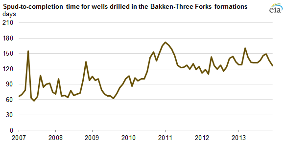
First, regarding rig productivity, the EIA points out that spud-to-completion times have actually increased to 120 days or more in the Bakken (Figure 1), a roughly 50% rise from four years ago. So even if it takes a few less days to drill a well, by the time it is fracked and tied into a pipeline the elapsed time has actually been getting longer. The so-called “fracklog”, which in the Bakken is estimated at 800-1000 wells, will likely increase spud-to-completion times (and cost) when the oil price rises enough to justify finishing the wells as there will be considerable competition for fracking crews.

Figure 1 – Spud-to-completion time for wells in the Bakken play of North Dakota and Montana (EIA).

 

The allegations of vastly improving well productivity due to technology innovations in shale oil plays such as the Bakken and Eagle Ford are examined below using the latest well production data.

Bakken Play

Figure 2 shows all wells in the Bakken Play by the month and year they were drilled. Each well is represented by four separate dots, indicating average daily production over its highest month (red), first 6 months (yellow), first 12 months (green), and first 24 months (blue). The lines indicate average daily production for all wells at these same points in time of well life (polynomial best-fit trend lines). This figure indicates that:

• Although there are a few very good wells with peak month production of over 1000 barrels per day, the average is about 500 barrels per day and is trending down, despite the application of ever-better technology.
• There is no observable increase in productivity in 2014 as widely reported. In fact, well productivity as defined by highest-month production peaked in mid-2014 and is declining.

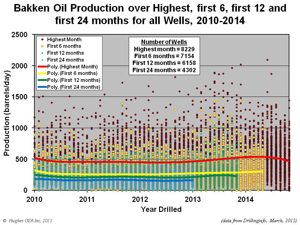
Figure 2 – Average daily production for all wells drilled in the Bakken Play between 2010 and November 2014. Dots indicate production over each well’s highest month (red), first 6 months (yellow), first 12 months (green), and first 24 months (blue). Lines indicate average daily production for all wells at these same points in time of well life (polynomial best-fit trend lines).

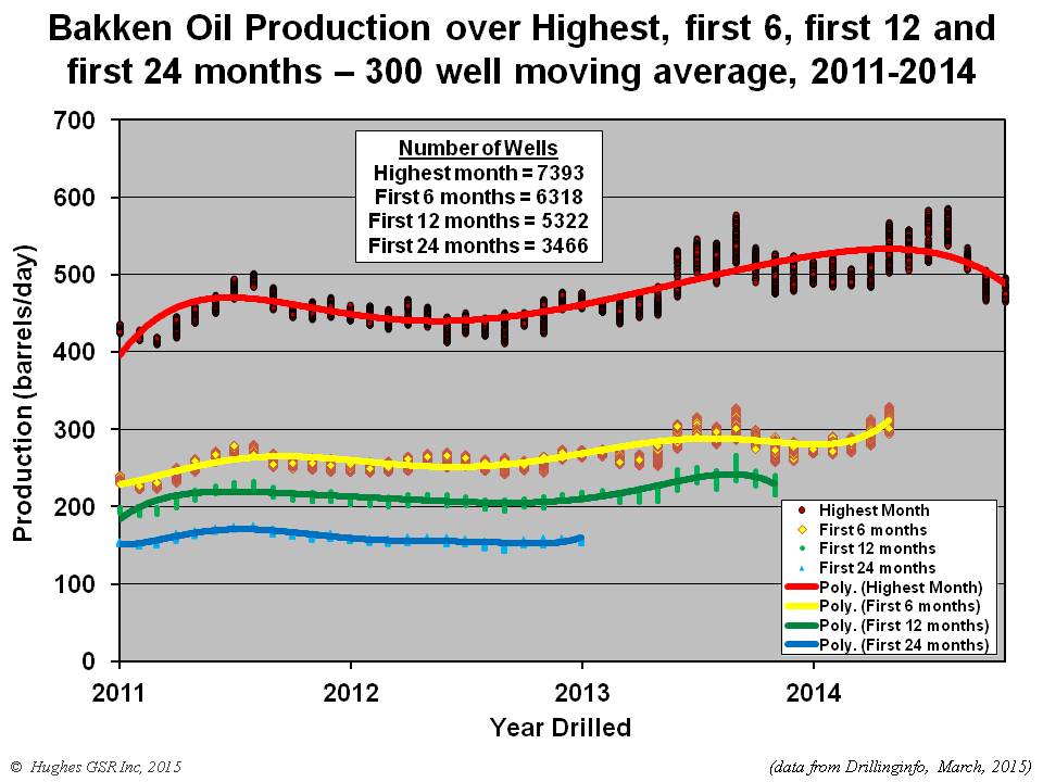
Figure 3 accentuates trends in well productivity in the Bakken by fitting a moving average to the data.  This figure indicates that:

• Significant improvements in well productivity were attained between mid-2012 and late-2013. This is a testament to both better technology and focussing on sweet spots.
• Productivity has stagnated since late-2013 and has fallen sharply in the last half of 2014.
• Highest month productivity is a key indicator of productivity over the longer term, as it is reflected in 6 month-, 12 month- and 24 month-average production.
• Production over the first 24 months peaked in mid-2011.

Figure 3 – Average daily production for all wells drilled in the Bakken Play between 2011 and November 2014. Data have been fitted with a trailing 300-well moving average to make the trends more apparent. Dots indicate production over each well’s highest month (red), first 6 months (yellow), first 12 months (green), and first 24 months (blue). Lines indicate average daily production for all wells at these same points in time of well life (polynomial best-fit trend lines).

 

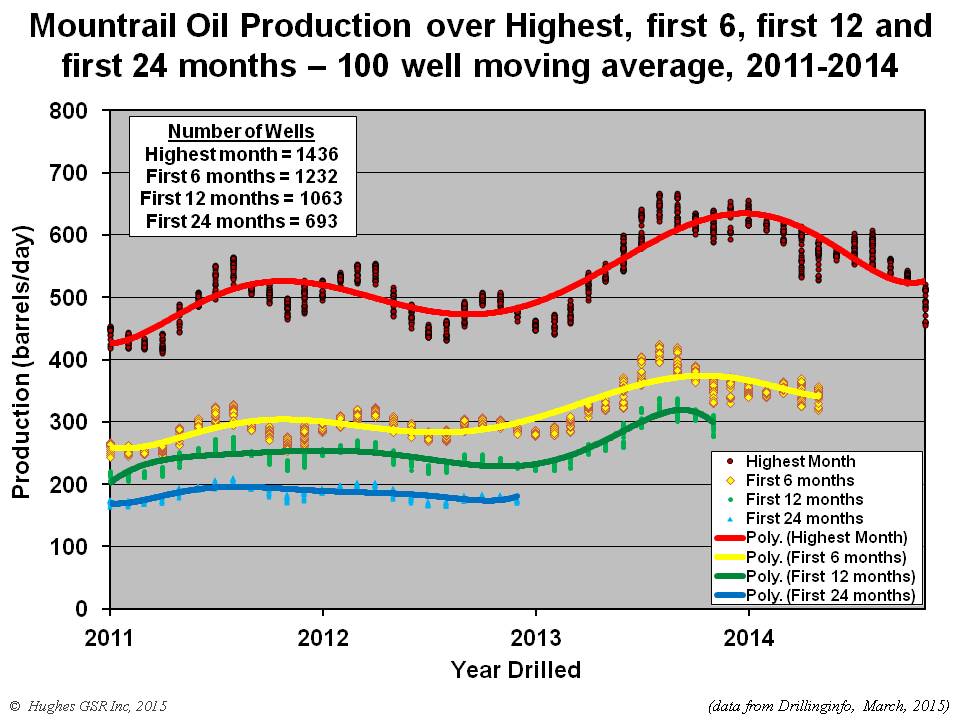
A key question covered in company investor presentations in the Bakken regards well downspacing: how close can wells be spaced and still increase total oil recovery? The Bakken is far from uniform in terms of well quality (see Figure 2-10 in Drilling Deeper), and four of 15 counties have produced 80% of the oil. Mountrail County has been the top producer so far, accounting for the largest share of cumulative production. Figure 4 illustrates average well production in Mountrail County over various periods. This figure indicates that:

• After a steep ramp up in highest month well productivity in 2013 productivity peaked and has now declined by nearly 20%.
• The fall off in well productivity is likely due to the density of current drilling, resulting in early signs of well interference, and to drilling more marginal parts of the county.
• Despite the hype by industry and drilling equipment purveyors, geology is already trumping technology in Mountrail County, which was the best of the best in terms of sweet spots in the Bakken Play. Well density in the prospective part of Mountrail County was 1.71 wells per square mile in mid-2014 (see Table 2-1 in Drilling Deeper) and well interference is already becoming apparent (I had assumed the entire Bakken could be drilled to 3 wells per square mile for my projections in Drilling Deeper, so I may have been a bit too optimistic).
• The assertions of increasing productivity are not true in this most productive and intensely drilled portion of the play – in fact productivity is declining. The happy talk is just that, and shouldn’t be relied on in terms of projecting the future of Bakken production.

Figure 4 – Average daily production for all wells drilled in Mountrail County of the Bakken Play between 2011 and November 2014. Data have been fitted with a trailing 100 well moving average to make the trends more apparent. Dots indicate production over each well’s highest month (red), first 6 months (yellow), first 12 months (green), and first 24 months (blue). Lines indicate average daily production for all wells at these same points in time of well life (polynomial best-fit trend lines).

 

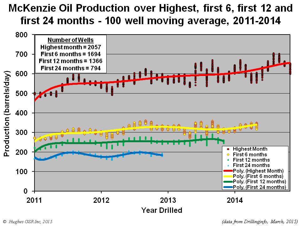
McKenzie County has recovered the second largest amount of oil in the Bakken Play and has the largest prospective area of any county. It is the only county exhibiting an upward trend in well productivity as illustrated in Figure 5. This figure illustrates that:

• Well productivity in terms of the highest month has increased significantly over the 2011-2014 period, but assertions that there has been a 29% increase in the past year are unfounded.
• Recent highest month well productivity has been declining and production over the first 6-, first 12- and first 24-months have been essentially flat since mid-2012, again belying assertions of substantial increases.
• In mid-2014 McKenzie County’s prospective area had only been drilled to 1 well per square mile so it is in an earlier phase of development than Mountrail County, but will certainly encounter the same downward spiral in well productivity through interference and drilling lesser quality locations as drilling density increases.

Figure 5 – Average daily production for all wells drilled in McKenzie County of the Bakken Play between 2011 and November 2014. Data have been fitted with a trailing 100 well moving average to make the trends more apparent. Dots indicate production over each well’s highest month (red), first 6 months (yellow), first 12 months (green), and first 24 months (blue). Lines indicate average daily production for all wells at these same points in time of well life (polynomial best-fit trend lines).

 

Bakken production is on track to follow the low drilling rate projection outlined in Drilling Deeper, although if drilling rates are reduced substantially below the minimum rates assumed in Drilling Deeper they will result in steeper declines initially and lesser declines later on.

Eagle Ford Play

Although there are nearly 12,000 producing wells in the Eagle Ford Play, analysis is complicated by the fact that the State of Texas reports production from multi-well leases as a single value. Hence only data from individual wells and one-well leases can be used for comparative analysis which, unfortunately, eliminates 40% of the producing wells in the play. Figure 6 illustrates the average production of all applicable wells in the Eagle Ford play over the highest month, and the first 6-, first 12- and first 24-months of well life. This is on a “barrels of oil equivalent” basis counting gas production as its energy equivalent to oil, given that the gas is a very important component of Eagle Ford production (as well as being the top producer of tight oil, the Eagle Ford is also the nation’s third largest shale gas field). This figure indicates that:

• Although there are a few very good wells with peak month production of over 1500 barrels per day, the average is about 800 barrels per day and is trending down, despite the application of ever-better technology.

 

• There is no increase in well productivity in 2014 of the magnitude alleged by the EIA. In fact, well productivity as defined by highest month production peaked in mid-2014 and is declining.

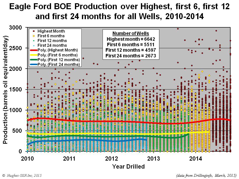
Figure 6 – Average daily production for all wells drilled in the Eagle Ford Play between 2010 and November 2014. Gas has been converted to oil on an energy equivalent basis (6000 cubic feet of gas equals one barrel of oil). Dots indicate production over each well’s highest month (red), first 6 months (yellow), first 12 months (green), and first 24 months (blue). Lines indicate average daily production for all wells at these same points in time of well life (polynomial best-fit trend lines).

Figure 7 accentuates trends in well productivity in the Eagle Ford by fitting a moving average to the data.  This figure indicates that:

• Significant improvements in well productivity were attained between mid-2013 and mid-2014. This is a testament to both better technology and focusing on sweet spots.
• Peak month productivity has stagnated since mid-2014 and is now falling.
• Highest month productivity is a key indicator of productivity over the longer term, as it is reflected in 6 month-, 12 month- and 24 month-average production.
• Productivity over the first12- and first 24-months has stagnated since mid-2011. Productivity over the first 6 months has increased slightly through early 2014 but is now falling.

Figure 7 – Average daily production for all wells drilled in the Eagle Ford Play between 2011 and November 2014. Data have been fitted with a trailing 300 well moving average to make the trends more apparent. Dots indicate production over each well’s highest month (red), first 6 months (yellow), first 12 months (green), and first 24 months (blue). Lines indicate average daily production for all wells at these same points in time of well life (polynomial best-fit trend lines).

 

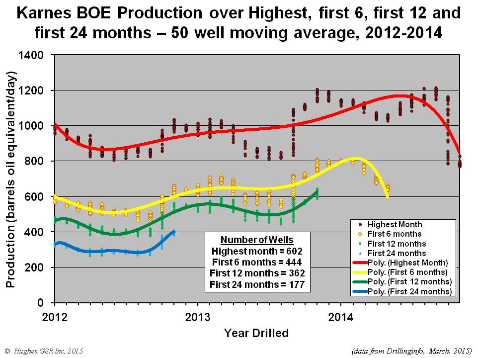
As in the Bakken, a key tenant of company investor presentations in the Eagle Ford is downspacing – how close can wells be spaced and still increase total oil recovery. The Eagle Ford is far from uniform in terms of well quality (see Figure 2-29 in Drilling Deeper), and six of 28 counties have produced 80% of the oil. Karnes County has been the top producer so far, accounting for the largest share of cumulative production. Figure 8 illustrates average well production in Karnes County over various periods. This figure indicates that:

• After a steep ramp up in peak month well productivity in 2013, productivity was essentially flat through mid-2014 and has declined 30% in recent months.
• Decline in first 6 month productivity is even steeper than peak month for the same wells. The fall off in well productivity is likely due to the density of current drilling, resulting in well interference, and to drilling more marginal parts of the county.
• Despite the hype by industry and drilling equipment purveyors, geology is already trumping technology in Karnes County, which has to date produced the most oil in the Eagle Ford Play. Well density in the prospective part of Karnes County was 2.76 wells per square mile in mid-2014 (see Table 2-2 in Drilling Deeper) and well interference is already becoming apparent (I had assumed the entire Eagle Ford could be drilled to 6 wells per square mile for my projections in Drilling Deeper, so I may have been a bit too optimistic).
• The assertions of increasing productivity are not true in this most productive and intensely drilled portion of the play – in fact productivity is declining. The happy talk is just that, and shouldn’t be relied on in terms of projecting the future of Eagle Ford production.

Figure 8 – Average daily production for all wells drilled in Karnes County of the Eagle Ford Play between 2012 and November 2014. Data have been fitted with a trailing 50 well moving average to make the trends more apparent. Dots indicate production over each well’s highest month (red), first 6 months (yellow), first 12 months (green), and first 24 months (blue). Lines indicate average daily production for all wells at these same points in time of well life (polynomial best-fit trend lines).

 

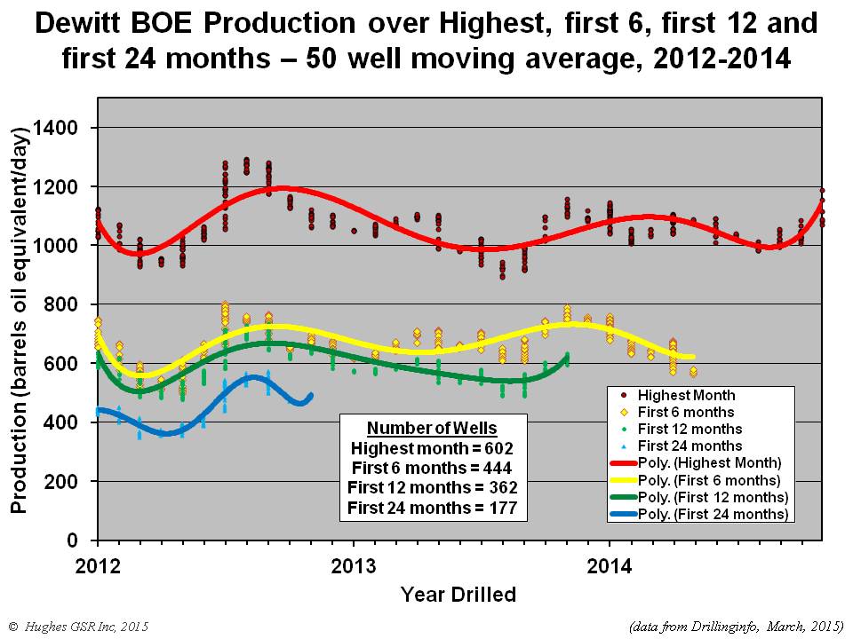
The Eagle Ford is larger than the Bakken, both in terms of overall areal extent and in the size of the core area. As well as Karnes County, Dewitt, Lasalle, Dimmit, Gonzales and McMullen counties have also been prolific producers. An example of well productivity trends for Dewitt County is illustrated in Figure 9. This figure illustrates that:

• Well productivity in terms of the highest month peaked in mid-2012 and has been relatively flat since late-2013. There is no indication of a significant ramp up in productivity over the past year as widely reported.
• Well productivity over the first 6 months has been declining since late 2013, even though highest month productivity has been relatively flat over the same period, suggesting potential early signs of well interference. Well productivity over the first 12- and first 24-months peaked in mid-2012.
• Dewitt County has been drilled to just over 3 wells per square mile. Counties such as Lasalle, Dimmit, Gonzales and McMullen have been drilled at between 1.36-2.18 wells per square mile so are in earlier phases of development than Karnes or Dewitt counties.  

Figure 9 – Average daily production for all wells drilled in Dewitt County of the Eagle Ford Play between 2012 and November 2014. Data have been fitted with a trailing 50-well moving average to make the trends more apparent. Dots indicate production over each well’s highest month (red), first 6 months (yellow), first 12 months (green), and first 24 months (blue). Lines indicate average daily production for all wells at these same points in time of well life (polynomial best-fit trend lines).

 

Some 30,000 wells remain to be drilled in the Eagle Ford before it is fully saturated. The trends in well productivity so far suggest that the best days are right now, and may already be behind us in top counties like Karnes. There has been no technology “big win”, as widely believed, and well productivity will decline as the best areas become saturated and drilling moves into lower quality rock. The recent decline in rig count suggests drilling rates may fall below the “low” projection in Drilling Deeper, resulting in an earlier peak followed by a longer plateau and slower ultimate production decline for the play as a whole. 

Summary and Implications

Central points from this analysis include:

• Irrespective of price, geology is trumping technology in the Bakken and Eagle Ford plays.
• The widely reported ramp up in well productivity in the Bakken and Eagle Ford plays over the past year due to technology improvements does not exist when examined at the play- and county-level . Although some operators may have experienced productivity increases depending on the location and quality of their leases (eg. Whiting in Mountrail County of the Bakken), others have experienced correspondingly greater than average decreases.
• Well productivity in the top-producing counties of both the Bakken and Eagle Ford is declining, despite the application of the best technology. This is due both to saturation of the best parts of these counties with wells and resultant movement to lesser quality areas, and potentially to well interference as densely spaced wells cannibalize each other’s production.
• The decline in well productivity in top counties is particularly disturbing given the incentive for operators to move drilling into core areas to maximize economics given the drop in oil price.
• The widely speculated decline in shale oil production due to the fall in rig counts will not become fully evident in actual production data for a few months, due to the typical 2-4 month lag in data release, along with inevitable revisions.
• The drop in rig count will certainly affect near term production but will not significantly change the amount of oil that can ultimately be recovered from these plays. In fact it will save oil for later, reducing the post-peak rate of production decline.
• The industry’s propensity to drill its best locations first means that prices will have to go much higher to recover the last of the oil from these plays.
• Projections in Drilling Deeper may be a bit too optimistic in the short term given the decline in rig count and associated drilling rate but are on track for the longer term.