
An ocean of ink has already been spilled on pros and cons of using Hubbert curves to model production from a large collection of wells in one or many reservoirs. In 2010, I published together with my last graduate student in Berkeley, Dr. Greg Croft, a highly cited paper on this subject. I have also commented multiple times in this blog on the different aspects of the Hubbert curve analysis, its limitations, and predictive power.
Since I cannot out-talk or out-convince the numerous critics of this type of analysis, let me give you a simple example of its robustness. This particular story is as follows. At the end of the year 2010, Greg Fenves, at that time Dean of UT’s Cockrell School of Engineering in Austin, asked me to make a presentation to the School’s Engineering Advisory Board (EAB). Using the results of our recent paper with Greg Croft, I chose to speak about my new work on unconventional resources in the U.S. On April 09, 2011, I made the presentation, which was then internally published by the Cockrell School.
The first two Barnett shale plots shown below were based on the Texas Railroad Commission data through October 2010. In the presentation, I called these plots the "high production scenario." The Hubbert curve with which I matched the production data ending in October 2010, went right between the two local peaks of the data. Of course there was an element of luck, helped by two decades of my experience as a reservoir engineer. Such experience or – for that matter – any other knowledge of reservoir engineering is absent among the economists, political scientists and journalists, who are paid to criticize this type of work.
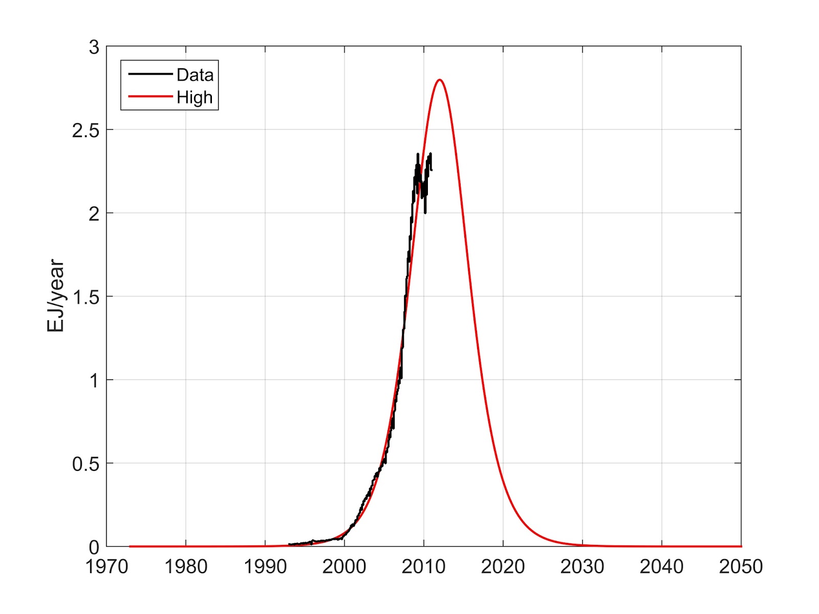 |
| To see this image in full resolution, please click on it. The total rate of gas production in the Barnett shale through October 2010, was matched with a single Hubbert curve. 1 EJ/year ~ 1 trillion standard cubic feet (TCF)/year. This "high production case" was presented in April 2011, at the Spring meeting of the Cockrell School Engineering Advisory Board (EAB) at the University of Texas in Austin. It was also made available electronically to the EAB members. |
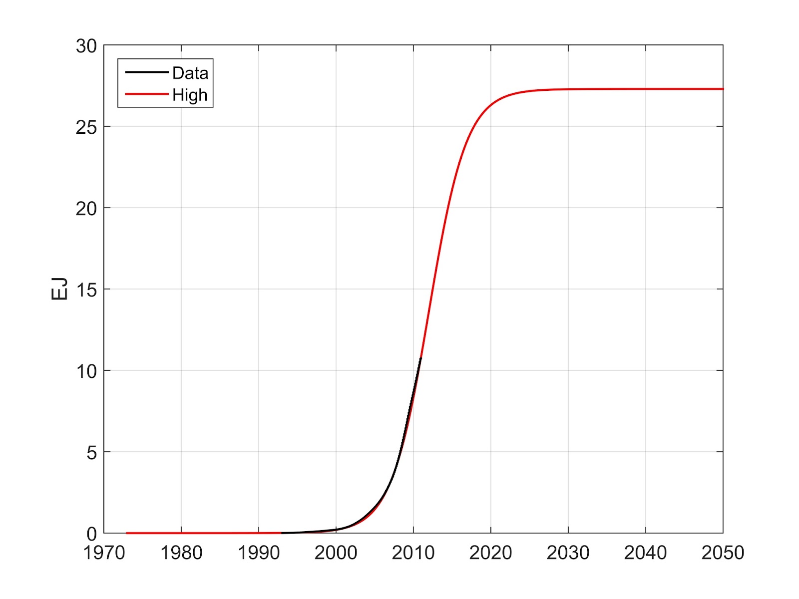 |
| To see this image in full resolution, please click on it. Cumulative gas production in the Barnett shale through October 2010, was matched with a single Hubbert curve (an integral of the bell curve shown above). The projected ultimate production was at least 27 TCF. 1 EJ/year ~ 1 TCF/year. |
In fairness to lay people, the respected reservoir engineers who saw these curves in 2011, smiled at my naïveté and predicted 60, 100 plus, or more TCF of gas production from the Barnett. In short, most experts were also amused.
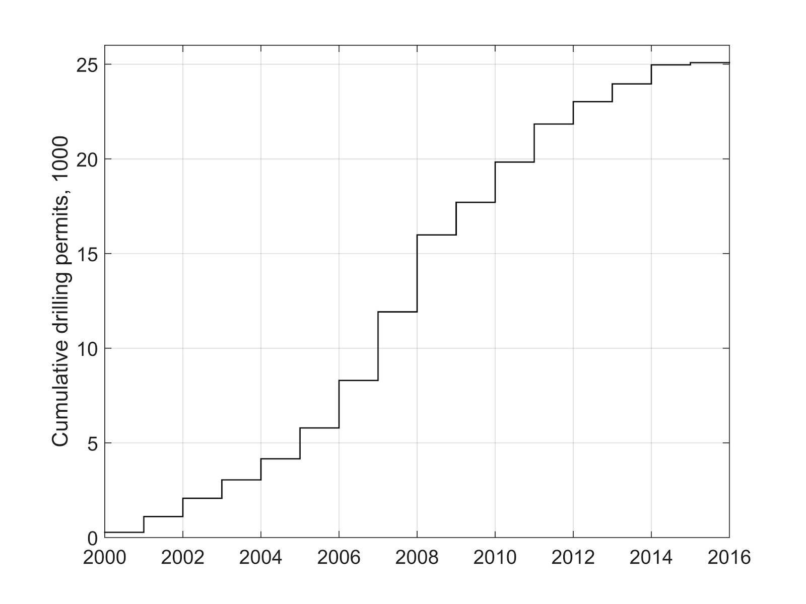 |
| Cumulative drilling permits issued by the Texas Railroad Commission for (the mostly horizontal) wells in the Barnett shale. Note that the cumulative permit curve follows a logistic S-curve similar to the cumulative gas production above, only shifted in time. Peak wells (4,065 at the inflection point in 2008) were drilled ahead of peak gas production in 2012. We are beginning to see the ultimate "carrying capacity" of past drilling in the Barnett. To change this S-curve, we need a brand new Hubbert cycle of drilling. |
What did I do? I used a two parameter curve (height and width) to describe and extrapolate production from close to 20,000 wells in the Barnett. I knew two things: (1) this production could be matched with one Hubbert curve or 2-3 of them, and (2) I had to go above current gas production (overshoot it) because this production had not already peaked. The first observation is based on the Central Limit Theorem explained in our paper, and the second one is an admission that more wells will be drilled and production will increase further, we just do not know by how much. Experience and intuition allow one to reasonably guess the size of this production increase. Guessing is an art and not all experts are artists.
 |
| To see this image in full resolution, please click on it. The total rate of gas production in the Barnett shale through March 2015, is matched with a single Hubbert curve. 1 EJ/year ~ 1 trillion standard cubic feet (TCF)/year. |
To see how good this December 2010 prediction was, fast forward five years. I should remind you that the Hubbert cycle predictions of future production of a very large number of wells and/or reservoirs are remarkably stable – the Central Limit Theorem makes sure of this, but I would not be happy if I predicted gas production in the Barnett shale with a 50% error. Luckily, as the plot above shows, I was right on the money, and no corrections were needed. Nevertheless, I could not resist tweaking the peak almost imperceptibly and increased the ultimate gas production from the Barnett by less than 1 TCF. Call it a reservoir engineer’s decease.
 |
| To see this image in full resolution, please click on it. Cumulative gas production in the Barnett shale through March 2015, is matched with a single Hubbert curve. The projected ultimate production is at least 28 TCF. 1 EJ/year ~ 1 TCF/year. |
In summary, given the current number of wells in the Barnett shale (over 25,000 drilling permits by now) and the already traversed peak of gas production, it is unlikely that I will have to adjust this prediction in the future, but let me play devil’s advocate.
The Barnett shale is most unusual in that it has two sets of fractures in the hydrofractured rock surrounding horizontal wells. One set is formed by the stress relief cracks from shear rock failure during hydrofracturing. Think of these cracks as being almost parallel to main hydrofractures and extending some distance away from both sides of these hydrofractures. But the Barnett shale is also likely to have another set of critically stressed (ready to pop), cemented natural fractures perpendicular to the hydrofracture planes. Together these two sets of fractures link during hydrofracturing and form large complex fracture systems that also communicate with the main hydrofractures. Thus, one could use this wonderful property of the Barnett mudrock, not replicated in other major shales, to create in the future many better and cheaper wells in the Barnett. If this happens, I will add a new Hubbert curve to my Barnett shale production model to account for the new wells, and happily report a significant increase (but not by 50%) of gas production there.
 Shale gas sign teaser image via shutterstock. Reproduced at Resilience.org with pemission.