 What do you get when you cross an astronomically-inclined physicist with concerns over energy efficiency in lighting? Spectra. Lots and lots of spectra. In this post, we’ll become familiar with spectral characterization of light, see example spectra of a number of household light sources, and I’ll even throw in some mind-blowing photos. In the process, we’ll evaluate just how efficient lighting could possibly be, along the way understanding something about the physiology of light perception and the definition of the increasingly ubiquitous lighting measure called the lumen. Buckle your physics seat-belt and prepare to think like a photon.
Spectral Introduction
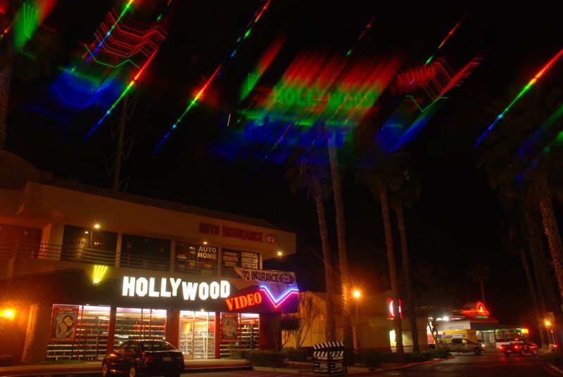
Figure 1: Abundance of sources, spectrally residing in the sky. The Hollywood sign is backlit by standard fluorescent tubes. A variety of other source types are discernible as well.
What do I mean by spectra? Light is characterized by wavelength, running from 400 nanometers (nm, or billionths of a meter) at the blue/violet end to 700 nm at the red end. Some familiar sources emit light at a single, pure wavelength—called monochromatic—like red helium-neon lasers at 633 nm, doubled-YAG (green) lasers at 532 nm, and those very orange low-pressure sodium streetlights at 589 nm (Figure 3). But most natural light sources (or colors) are composed of continuous distributions of light at all visible wavelengths. White light has a healthy helping of all colors, as can be seen in a rainbow, spanning red to violet.
Meanwhile, many synthetic lights (fluorescents; gas discharge tubes such as neon; mercury vapor and sodium vapor lights; etc.) emit a line spectrum—an amalgam of discrete wavelengths associated with atomic and/or molecular energy transitions, possibly with a bit of phosphor thrown in to give some modicum of continuum light.
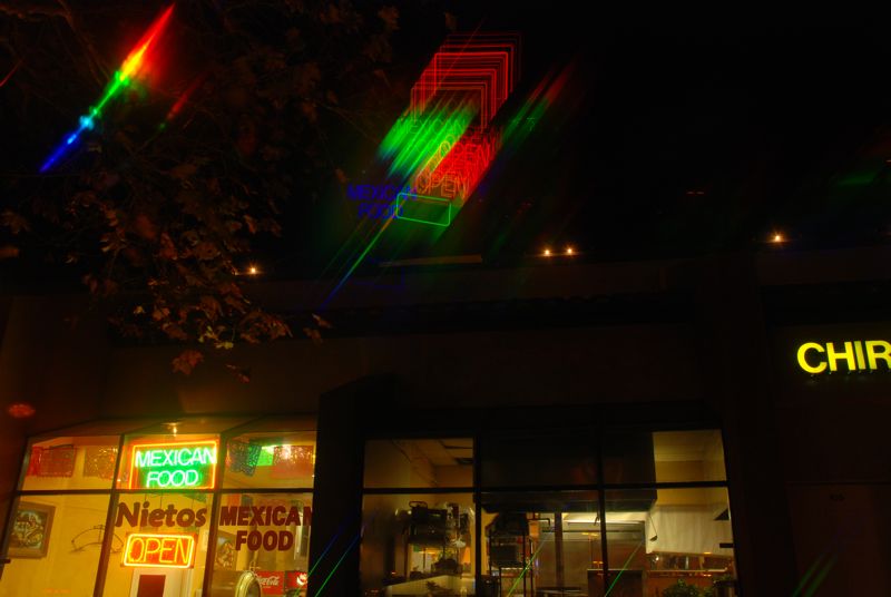
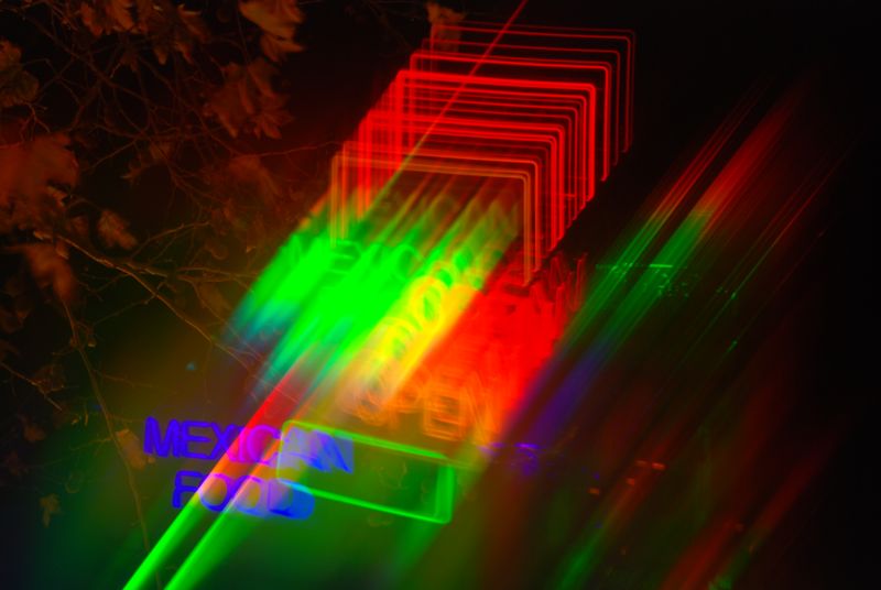
Figure 2: A pair of “neon” signs broken up into spectral components, top-center. The strong line/continuum spectrum at upper left is from a light out of the field of view.
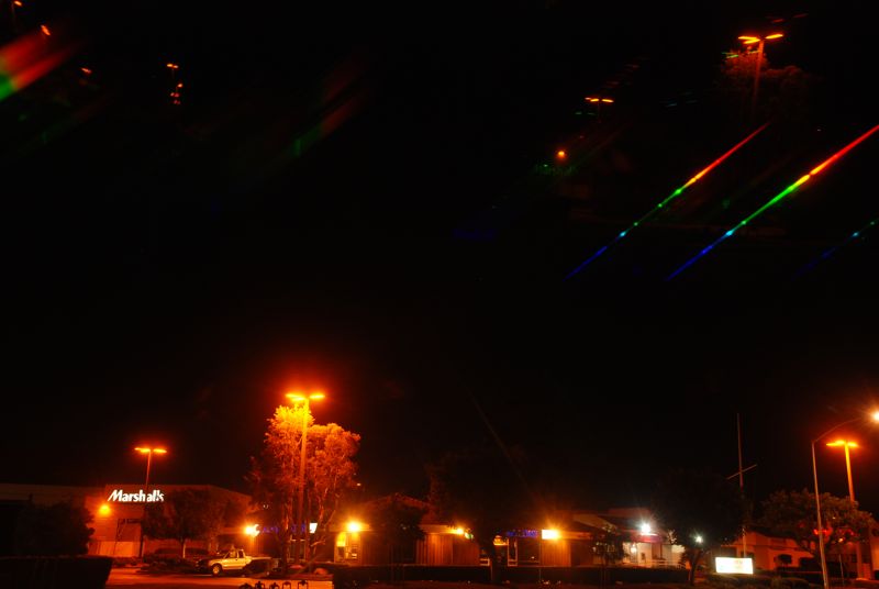
Figure 3: A low-pressure sodium vapor lamp over a tree is almost perfectly monochromatic, as seen by the single, sharp spectral image at upper right. A much weaker green line is also barely visible. Two other LPS sources in the lower-left of the picture are seen in their monochromatic spectral form near the upper-right.
Colored LEDs (light-emitting diodes, e.g., red, orange, green, blue; Figure 4) are in between the continuum and line sources, emitting light over a continuous—though not very broad—part of the spectrum. Maybe “fat line sources” would be a reasonable characterization.
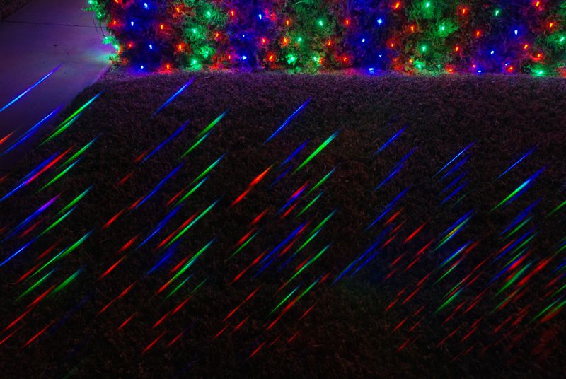
Figure 4: Colored LEDs each result in short spectra, almost pure in color. The green LEDs do extend a bit into the blue.
The photos above from around my neighborhood illustrate various forms of spectra in a rich, but sometimes bafflingly complex, way—obtained by placing a transmissive diffraction grating film in front of the lens. The combined-light (un-dispersed) scene is visible in each, but stretching off at an (arbitrarily-set) angle is the “dispersed” version of the same. Line sources produce replications of their shape at each emission wavelength, while continuous sources smear out. The distance from the un-dispersed source to its spectral replica is proportional to the wavelength of light (deep blue/violet is closer, at 400 nm, than deep red, at 700 nm). But the camera helpfully color codes these as well. Note that the low pressure sodium lights are essentially monochromatic—so make a single, sharp, replica at 589 nm. Gas-discharge tubes (as seen in Figures 1 & 2 and intro figure) have a forest of lines. Meanwhile, the colored decorative LED lights produce short, stubby spectra in their “fat monochromatic” way (Figure 4).
Color Perception
Our eyes are essentially tri-color devices. If you look at a sharp spectrum of white light (a rainbow is too mushy, with overlapping colors), you mainly see red, green, and a blue-violet: not much yellow or cyan between the colors. It is only in combination that we create mixture colors. This is why an RGB monitor can synthesize almost any color by varying the brightness of red, green, and blue pixels. Figure 5 shows a representation of the visual spectrum that is not far from our perception, showing the sensitivity curves of the three color receptors in the eye. When we perceive L > M, we call it red, and if we sense L < M, we call it green—until S starts to perk up. I am guessing the S, M, and L labels mean short, medium, and long wavelength.
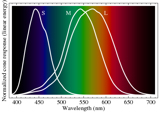
Figure 5: Tri-chromatic sensitivities imposed on visible spectrum.
As an aside, if I generate a sharp, continuous solar spectrum for my camera, I see a similar tri-color behavior—albeit much more faithfully red-green-blue (Figure 6). These relate to the filters used in front of the pixels to sort out light by color. Note the absence of very much yellow or cyan in the transitions from red to green and green to blue, respectively.
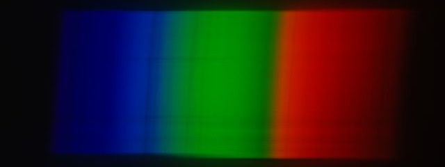
Figure 6: Solar spectrum (through slit) captured with the same camera and grating as the other photographs. Not much yellow or cyan to be seen, reflecting sharp filter cutoffs. Absorption lines (Fraunhofer lines) are visible in the spectrum, arising from constituents in the solar atmosphere.
In aggregate, our visual sensitivity peaks in the green, at 555 nm, falling off on either side in something called the photopic function (there is also a scotopic function for night vision—rods rather than cones—shifted a bit toward the blue). Figure 7 shows the photopic sensitivity function (blue), with a solar-temperature blackbody curve (black) and an incandescent filament blackbody curve (red) also shown for reference.
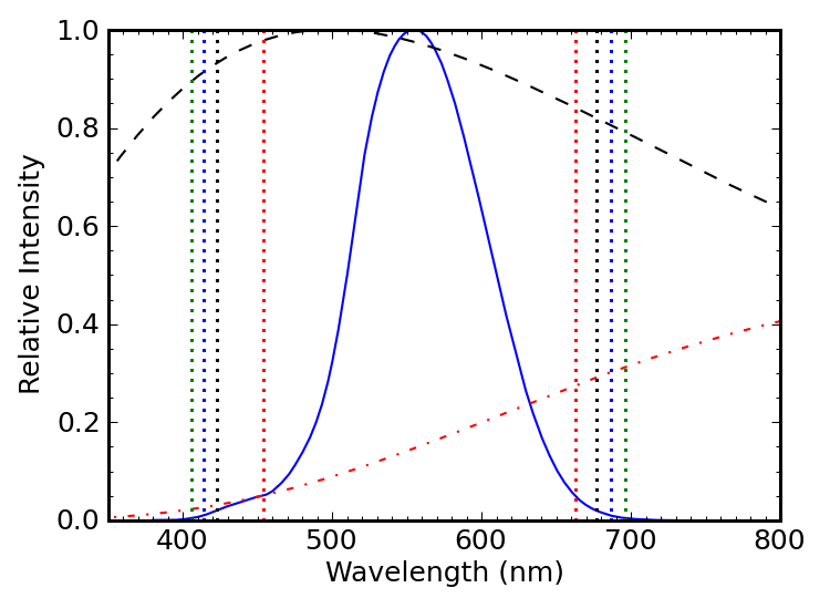
Figure 7: The photopic sensitivity curve (blue) compared to the solar blackbody spectrum (black) and a blackbody at a temperature characteristic of incandescent bulbs (red).
I will be referring to blackbody spectral distributions, also called Planck functions, after Max Planck. Don’t take the word “black” literally here: think of it as “dull,” as in not shiny like metal. Any “dull” object emits thermal radiation (shiny ones do too, but at suppressed strength). As the temperature climbs, the radiation shifts from the infrared into visible wavelengths, so that a poker may get red-hot; coals get orange-hot, and the Sun is white-hot. These are all blackbodies, and we generally strive to emulate them in our artificial lighting sources. Incandescent bulbs cleverly manage to do this by actually being hot, radiating blackbodies. Their only problem is that most of the light is generated outside of the visible domain. More on this later.
The Lumen
The lumen is a unit that captures how bright a source appears to the human eye. A laser pointer putting out 5 mW of light at 532 nm (green) will emit 3 lumens (lm) of light, while a red laser pointer at 633 nm emitting the same amount of power is only seen to be 0.8 lm. Meanwhile, an infrared laser of any (modest) power output will register zero lumens, since the eye cannot perceive its brightness.
Every photon of light carries a discrete amount of energy, in Joules: E = hc/?, where h = 6.626×10⁻³⁴ J·s is Planck’s constant, c ≈ 3×10⁸ m/s is the speed of light, and ? is the wavelength of the photon, expressed in meters (green light is about 5.5×10⁻⁷ meters, or 550 nm). So a stream of photons emerging from a light can be associated with a power, measured in Watts, since we can specify how many photons per second are emitted, each carrying known energy. Energy per time is power, and Joules per second is also called Watts.
The lumen is defined so that at the peak of the photopic sensitivity curve (555 nm), one Watt of photon power will carry a brightness of 683 lumens. We can then describe the luminous efficacy of a monochromatic 555 nm source as 683 lumens per Watt (lm/W).
If you stand in front of a selection of light bulbs at the store, you should be able to find the brightness in lumens listed somewhere on the box. You’ll also usually find the actual power consumed by the light bulb. In the case of fluorescent or LED lights, this is not the “replacement wattage” in incandescent terms, but the actual electrical power consumed when the device is on. Dividing these numbers, you’ll find that incandescent lights have luminous efficacies around 15 lm/W. Fluorescent and LED lights tend to be closer to 60–80 lm/W. Much better, but far short of our 683 lm/W monochromatic green source.
Luminous Efficacy of Incandescents
You can figure out the luminous efficacy of any monochromatic (laser) source by gauging how high the photopic curve is at that wavelength relative to the peak, and multiplying this fraction by 683. But what about a distribution? In this case, an integral (piecewise sum of wavelength slices) of the photopic curve times the source spectrum in question does the job.
Incandescent lights are essentially blackbody radiators (glowing white-hot), whose spectra are described by the Planck function. Two examples are shown in the plot above, corresponding to the 5800 K surface temperature of the Sun and the 2800 K effective temperature of a light bulb filament. Incandescent lights are phenomenally efficient at converting electricity into photons. The problem is that most of those photons are emitted in the infrared portion of the spectrum, beyond human perception. A 5800 K blackbody emits 37% of its light between 400–700 nm, while only 6% of the light from a 2800 K filament comes out in the visible range.
We can ask what the luminous efficacy of a blackbody source of photons would be. It must be less than 683 lm/W, since many of the Watts are expended at wavelengths of low (or no) photopic sensitivity. The plot below (Figure 8) shows the result. The peak occurs at 6640 K and 96 lm/W, whereas the efficacies at 5800 K and 2800 K are 93 lm/W and 15 lm/W, respectively. Obviously, the solar spectrum achieves near-maximal efficacy. It’s no coincidence: our eyes are adapted to spectrum of our star.
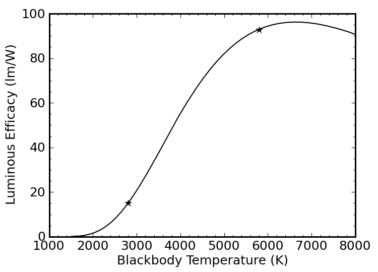
Figure 8: Luminous efficacy of pure blackbody sources.
So we could make incandescents more efficient by getting them hotter. The problem is that filaments melt if you get them much hotter than they are already. Halogen bulbs surround the filament with gases that redeposit evaporated atoms back onto the filament, letting them operate at slightly higher temperature. But even these are still far down on the curve.
How Good Can it Get?
Okay, so a blackbody source near 6000 K like the Sun gets up to nearly 100 lm/W. But how good would an ideal white light source be if we could engineer its spectrum to be anything we want? A quick-and-dirty answer can be had by using the fact that 37% of the solar spectrum is within visible limits. If we could design a source to mimic the solar spectrum, but emit not one photon of light at wavelengths we can’t see, we’d get something like 93/0.37 ≈ 250 lm/W.
We can refine this somewhat by recognizing that the eye’s sensitivity at the extreme ends of the visible spectrum (400 nm and 700 nm) is not so hot, so we could truncate our blackbody spectrum more aggressively, and get a higher luminous efficacy by wasting fewer photons where we need them less. The four sets of vertical dotted lines in Figure 7 above represent cutoffs at the 0.5%, 1%, 2%, and 5% levels of the photopic sensitivity curve (blue). In other words, if we were willing to limit the spectrum of our light source to wavelengths at which our eyes have at least 5% of the peak sensitivity, we’d be dealing with the range between the red dotted lines, from about 450–660 nm.
How high will the luminous efficacy climb as we narrow the range? Figure 9 tells the story.

Figure 9: Luminous efficacy achievable with truncated blackbody, as a function of truncation degree.
The efficacy gets better and better as we decrease the range. Ultimately, as we approach a cutoff at the 100% sensitivity level, we would be looking at monochromatic light at 555 nm, and a luminous efficacy of 683 lm/W. But this light is useless for color rendering: it’s just green.
So truncating the spectrum comes at a cost. Color rendering will not be as good when we drop the deep reds and deep violet/blues from the spectrum. If we’re going to cut corners for the sake of efficiency, we need to also evaluate the quality of color rendering to establish criteria for an acceptable white light source.
Color Rendering Index
There is a heinously twisted procedure by which one can evaluate the color rendering index (CRI) of a light, given its spectrum. I’ll spare you the details (and secretly wish I had also been spared), but essentially it boils down to “illuminating” eight specially-selected sample color swatches—not particularly attractive colors, I must say—with the test spectrum, and comparing the proximity in color space (think color wheel) to what would happen if the same source were illuminated by a blackbody (incandescent) at the same effective (color) temperature.
Terms that I will be using:
- CRI: Color Rendering Index; ranging from 0–100, with 100 representing perfect blackbody (incandescent) performance.
- CCT: Correlated Color Temperature; the blackbody temperature that results from illuminating a white source. Really, it’s the temperature of the closest blackbody point (called the Planckian locus) in color space. The sun has a CCT of 5800 K, while a typical incandescent bulb is around 2800 K—appearing redder. Higher CCT values look blue, like the light from the stars Sirius or Rigel. This ordering runs counter to intuitive labeling of redder light as “warm” (like fire) and bluer light as “cold” (like ice).
- Planckian Offset: related to CCT, the distance in color space to the nearest blackbody point (on the Planckian locus). Beyond a value of 0.0054, the source is considered to be too far from a blackbody to be considered “white,” and the computed CRI begins to lose meaning.
So if we explore the very best we can do in a truncated solar-type spectrum (CCT = 5800 K)—this time allowing red and blue cutoffs to be at differing photopic sensitivity cutoffs—we arrive at the following plot (Figure 10):

Figure 10: Maximum performance of a truncated 5800 K blackbody as a function of allowable color rendering performance.
How do we interpret this? Following the solid curve, at the right hand side, we can get a near-perfect CRI around 100 while achieving 260 lm/W. As we increase the level of spectral truncation, the luminous efficacy shoots up (not wasting photons on zones of weak sensitivity), but the CRI declines. Now looking at the dashed line, we find that we exceed the tolerable “white” limit (Planckian offset) of 5.4×10⁻³ at a CRI of 94 and a luminous efficacy of 310 lm/W. It turns out that this limit corresponds to a wavelength range of 423–659 nm. Thus 310 lm/W is the maximum luminous efficacy for a light we would still regard as “white” at the color temperature of the Sun.
At 2800 K, corresponding to the “warm” illumination to which we are accustomed, we actually do better (Figure 11).
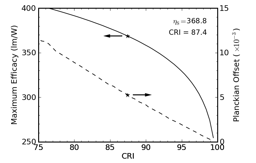
Figure 11: Maximum performance of a truncated 2800 K blackbody as a function of allowable color rendering performance.
Now, we slide all the way up to about 370 lm/W before busting the Planckian offset threshold, resulting in a CRI of 87 (a little shy of 90, but probably acceptable to most). The wavelength range in this case is 422–648 nm. The red-heavy 2800 K spectrum (see Figure 7) allows a bit more skimping on the red cutoff than was the case for the solar spectrum.
So if we could design a magic light source that emitted a blackbody-like spectrum across a finite wavelength range, generating photons at 100% electrical efficiency (such a source would not even be warm to the touch), we could hope to achieve luminous efficacy values in the range of about 300–370 lm/W. This is roughly a factor of five better than present sources, almost all because of electrical efficiency rather than spectral efficiency.
Example Spectra of Alternative Lights
Enough with the theoretical, magical light. What do real lights achieve? Below is a gallery of example spectra I acquired for various lights. Descriptions follow each one.

Figure 12: A compact fluorescent light (CFL) seconds after being turned on. The spectrum is dominated by line sources, with a forest of infrared lines that will later disappear.
Figure 12 shows a 16 W compact fluorescent light (CFL), billed as a “60 W” replacement, rated as producing 900 lumens (so 56 lm/W total). I caught this spectrum just after the light was turned on from a dead-cold state. The spectrum itself has a luminous efficacy of 283 lm/W, at a “warm” color temperature of 2600 K, a Planckian offset well below the 5.4×10⁻³ limit, and a not-so-stellar CRI of 83.
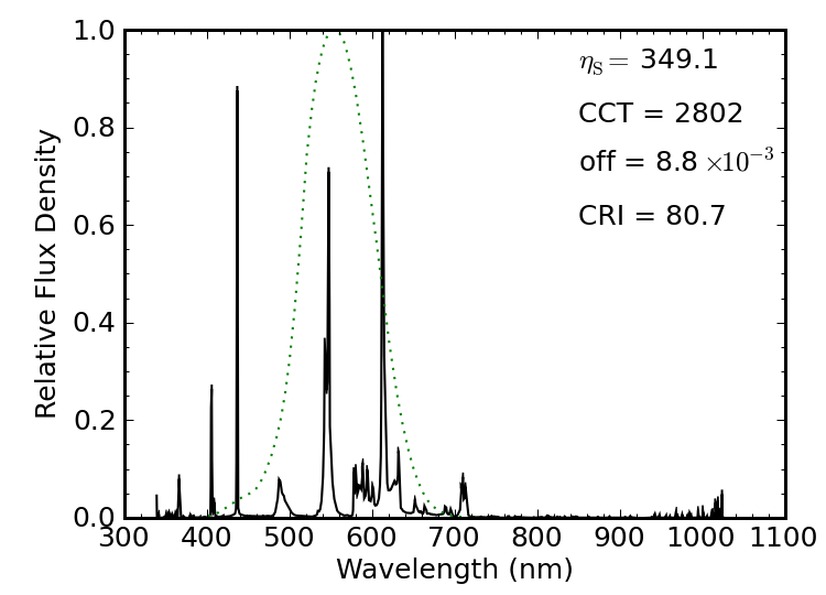
Figure 13: Same CFL bulb after warming up. Some semi-broad phosphors are used for continuum light, but lines still dominate.
The same bulb after a minute of warm-up has eliminated the forest of infrared lines, and has strengthened its green line relative to the others. The spectral luminous efficacy sails up to 350 lm/W on account of the fact that it no longer produces the infrared lines. But the source busts the Planckian offset limit, and the CRI sinks farther. The light certainly brightened considerably during the warm-up, even though the power draw (as measured via a kill-A-Watt) was steady at 16 W the whole time.
How do we reconcile the fact that a 900 lm source takes 16 W (56 lm/W) when the spectrum is cruising at 350 lm/W? Electrical efficiency. This CFL is turning only about 16% of its electrical energy into non-thermal photons. The photons it does produce are cleverly confined to the visible region (after warm-up), so its spectrum is about as efficient as one might like—even if the color rendering isn’t so hot—but the electrical-to-photon piece is the bottleneck.

Figure 14: A “warm” LED light spectrum. One blue LED pumps a broad-band yellow phosphor.
Figure 14 shows the spectrum of an LED light rated at 86 lm and sipping 1.5 W (about 60 lm/W). It’s color temperature is around 3000 K, and therefore “warm.” It’s really just a blue LED (narrow feature at left) pumping a broad yellow phosphor. The spectral luminous efficacy is quite high, at 340 lm/W, and its Planckian offset qualifies the source as being white. Its color rendering is pretty poor, however, at 66. Comparing the spectral luminous efficacy to the achieved luminous efficacy reveals a 17% efficiency at converting electrical energy into visible photons.
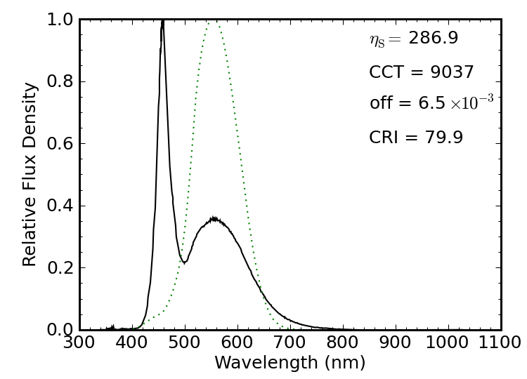
Figure 15: Similar to the bulb before, this LED light uses a blue LED to pump a broad-band phosphor, but less so.
A similar LED-based light advertised as having a color temperature of 6500 K is shown above, being just outside the “white” threshold, but having a better CRI (80) while turning in a poorer spectral luminous efficacy of 287 lm/W. The color temperature is measured to be much higher (“cooler”) than advertised. A similar blue LED is used in this light, but with much less of its light being absorbed and reprocessed by the phosphor. The packaging did not present the output in lumens, so I cannot evaluate the electrical efficiency.

Figure 16: Laptop screen illuminated by fluorescent light. Still line dominated, although the phosphors are broader than those used in the CFL bulb.
A laptop computer screen back-illuminated with a fluorescent source produces a solar-temperature spectrum that is very near the Planckian locus, and with respectable CRI (87) and a luminous efficacy of 317 lm/W. The main three line sources are the same as for the CFL bulb above, but the laptop screen makes more extensive use of phosphors, filling in the gaps between lines a bit more effectively.

Figure 17: Laptop screen illuminated by LED lighting. Same concept: blue LED pumps phosphors—in this case a green and a red.
A laptop screen back-lit by LEDs has the familiar blue LED pumping phosphors, but unlike the lights explored above, the laptop LEDs employ an additional phosphor to enhance illumination in the red part of the spectrum. The result is a borderline Planck-like spectrum “cooler” than the solar spectrum, and getting a CRI of 84. The spectral luminous efficacy is 293 lm/W. I also tried an LED-backlit television, with nearly identical results.
Finally, we have a cute device in our physics lecture demonstration facility at UCSD composed of three colored LEDs: one red, one green, and one blue. Three buttons allow any combination to be turned on, the light being thrown into a wedge of lucite (acrylic; plexiglass) with a roughened surface, so the lights diffuse and mix well. Push all three buttons, and you get a reasonable approximation to white. Red plus green (absence of blue) makes the primary subtractive color of yellow. Green plus blue (absence of red) makes cyan. Red plus blue (absence of green) makes magenta (Cyan, Magenta and Yellow—CMY—form the primary subtractive colors for dyes and paints). Sweet little toy. Given these three sources, what is the best mix (varying relative brightnesses) that maximizes the color rendering capability of the three in tandem?
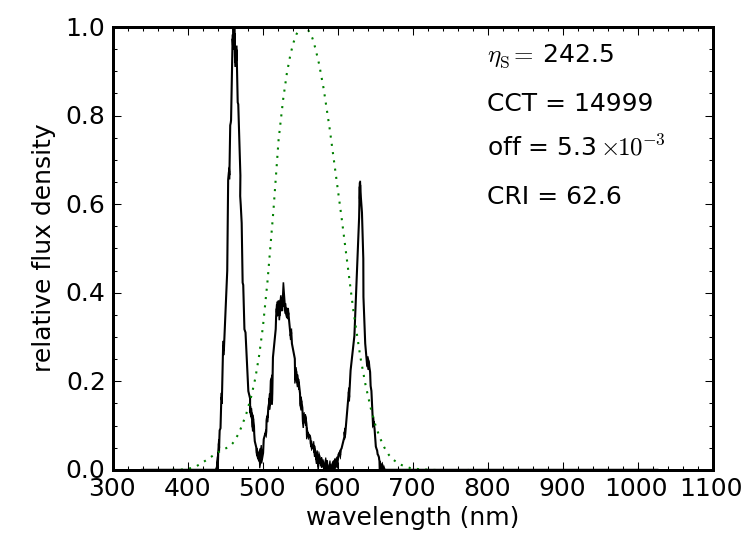
Figure 19: Three-LED (blue, green, red) mixture giving a white-ish light.
The best I could do is still not terribly good, by lighting standards. If I constrain the source to have an acceptably low Planckian offset, I only get a CRI of 63, and a luminous efficacy of 243 lm/W. If I allow any old offset from “white,” I can get the CRI as high as 77, but the offset is five times the “acceptable” limit (and luminous efficacy hardly budges—up to 246 lm/W). In both cases, the color temperature is absurdly high. The wavelengths of these three LEDs are not at all optimized for this task, so undoubtedly one could do better. Four LEDs (e.g., adding a yellow) would make it even easier.
Lessons
For most readers, this is way more than you ever wanted to know about light sources, spectral distributions, and maximum theoretical efficiency. I warned you at the beginning that this might happen when mixing astronomy and energy efficiency.
Besides being a sneaky way to educate folks about spectra, this post highlights that there is an absolute maximum efficiency achievable by lights. Every photon costs some energy. Even if we had a way of generating visible light photons at 100% efficiency, the photons themselves demand payment. Combined with our physiological sensitivity, and our judgment of suitable color rendering, we find that we will never exceed about 350 lm/W for lights that we would deem to be acceptable.
This means that present efficient lighting (spanning 60–100 lm/W) has only about a factor of four to go before reaching theoretical limits. As with many things, practical realities limit us to some fraction of the theoretical maximum. If we improved lighting efficiency at a rate of 2% per year (35 year doubling time), we would max out within the century.
Meanwhile, as we adjust to progress in lighting, we will find ourselves shaking off the old calibration of lighting intensity tied to Watts. The lumen is the right way to measure perceived brightness. If you keep in mind that standard incandescents are about 15 lm/W, then you can make the calibration yourself. A 1500 lm bulb is at the bright end. A reasonable general-purpose light might be around 600 lm. Flashlights can register in the tens of lumens. A recent excursion to look for LED headlamps demonstrated to me that the lumen is taking off as the primary figure of merit, with numbers typically ranging from 20 lm to 75 lm. I hope to see something like the CRI—and maybe even something akin to the Planckian offset—begin to play a role on the packaging as well, as consumers look for lights that have a natural feel. But who am I kidding? Silly rabbit: the only number people tend to care about is on the price tag.
Aside: The Story of Why
It’s perhaps worth a paragraph to explain why I went to all this trouble to evaluate the maximum theoretical efficiency of white light. It started with curiosity, which—as so often happens—quickly turned into a visit to Wikipedia. A nice table on the Luminous Efficacy page lacked the entry I wanted. So I computed a value for a perfect, truncated blackbody and stuck it in the table. A year or two later, I read a report that quoted a similar maximum, to my delight. I sought the source and found out that it was…me—or Wikipedia, in any case. Looking back at the page, I saw a “citation needed” note. I was surprised to discover that I could not find a published work detailing this maximum. Seeing this hole in the literature, I decided to plug it. A paper conveying much of the content found here is soon to be published in the Journal of Applied Physics. I thought I’d share the juicy parts with those of you having the stomach for this sort of thing. At the very least, it’s a nice collection of spectra of actual household light sources. And even if those bring you no joy, maybe the pictures will?