 If you want to make your house more efficient at repelling the unpleasantness outdoors (whether hot or cold), what should you do first? Insulate the walls? Insulate the ceiling? The roof? Better windows? Draft elimination? What has the biggest effect? While I have regrettably little practical experience tightening up a house (it’s on my bucket list), I at least do understand heat transfer from a physics/engineering perspective, and can walk through some insightful calculations. So let’s build a fantasy house and evaluate thermal tradeoffs at 1234 Theoretical Lane.
Heat Transport
There are only three ways for heat to travel: conduction, convection, and radiation. No other options.
Conduction
The power (energy per unit time) flowing across a material by conduction sensibly depends on the material properties (thermal conductivity, Κ), the thickness of the material, t, the area, A participating in the conduction (between the cold and hot environments), and the temperature difference, ΔT. Without much thought, you could construct the correct relationship for the power transported by conduction by figuring out how it should scale as we change one variable or the other: Pcond = ΚAΔT/t, where Κ is the thermal conductivity of the material, taking on units of W/m/°C in the metric system. For many building materials, Κ is in the range of 0.1–1 W/m/°C. A sheet of plywood, at the lower end of the range (Κ ˜ 0.12, measuring 4×8 feet, or 3 m²; t = 0.019 m, or 0.75 inches, thick) would conduct about 19 W per degree Celsius presented across it.
R-value
The building industry characterizes materials by their R-value, which in the U.S. has the unfortunate units of ft²·°F·hr/Btu. The SI equivalent is a slightly more tidy m²·°C/W. The R-value builds the thickness, t, into the measure, so the same material in twice the thickness will earn twice the R-value.
Relating to intrinsic properties of the material, Κ and t, RUS = 5.7×t/Κ in the U.S., or more simply, RSI = t/Κ overseas. Our plywood from before would be characterized as R = 0.9 in the U.S., or 0.16 internationally. Note that the R-value is independent of area. To get the power flow across a surface, in Watts, we replace the relation two paragraphs back with Pcond = 5.7×AΔT/RUS, or Pcond = AΔT/RSI.
Convection
Convection is at its core just conduction into a moving fluid, which then carries the heat away by simply wafting it along. Adjacent to any surface in a fluid flow is a boundary layer of fluid that clings to the surface, so that the thermal flow is controlled by conduction across the boundary layer. For air, Κ ˜ 0.02 W/m/°C, and boundary layer thickness is often in the neighborhood of a few millimeters, putting the effective R-value (US) in the neighborhood of 1.
Boundary layers aside, convection power should be proportional to the area exposed and to the temperature difference between the skin and the surrounding air. A constant of proportionality, h governs how vigorous the coupling is, and is effectively capturing the physics of the boundary layer (which depends on the flow rate, surface details, etc.). In any case, we get a relation Pconv = hAΔT. Typical situations might see h ˜ 2 W/m²/°C at indoor surfaces (“still” air), h ˜ 5 W/m²/°C for light airs outdoors, and perhaps 10 or 20 in windy conditions. If our 3 m² piece of plywood is at room temperature (20°C) and is placed in a freezing breeze with an h value of 5, each surface would lose energy at a rate of 300 W.
Note that we can relate h to the R-value in a generic equation that looks just like the conduction relation: P = hAΔT = 5.7×AΔT/RUS, in which case we can identify h = 5.7/RUS = 1/RSI. In this case, the light airs of the outdoors (h = 5) may be associated with RUS ˜ 1.
Radiation
Every object radiates electromagnetically. At familiar temperatures, this all transpires in the mid-infrared, peaking at a wavelength of 10 microns and petering out completely by 2 µm (meanwhile, human vision is 0.4–0.7 µm). The net flow, naturally, is from hot to cold, and obeys the relation: Prad = As(ehT4h – ecT4c), where s = 5.67×10⁻⁸ W/m²/K4. The e factors are emissivity values, ranging from 0.0 (shiny) to 1.0 (dull). The temperatures must be expressed in Kelvin, as the amount of radiation depends on the absolute temperature of the object. Subscripts denote hot and cold objects. We’ll ignore complications from non-uniform environments.
So our piece of plywood, at room temperature (293 K) in radiative contact with a surrounding world at 0°C (273 K) would see about 300 W pouring off each surface if emissivities are assumed to be nearly 1.0. Pretty similar to convection (a good rule of thumb).
A word about emissivity. Most things have very high emissivity. Anything organic (wood, skin, plastics, paint of any color) is likely to have an emissivity in the neighborhood of 0.95. Even glass, with a semi-shiny (partially reflective) surface is 0.87. Only shiny metals dip low, which is why ducts, some insulation, and thermos bottles employ shiny surfaces: to knock out the radiative heat loss channel.
Annoyingly, radiation is not just proportional to ΔT, being instead proportional to the difference between the fourth powers of the temperatures. However, for small temperature differences on the absolute scale (fortunately commonplace), we can linearize the relation (here assuming unit emissivity) to Prad ˜ 4AsT³ΔT, where the T in the cubic term is a representative temperature, perhaps between the hot and cold. Notice that the form now looks just like convection, with 4sT³ replacing h. For the foregoing examples, if we pick T = 283 K, we find an equivalent h-value of 4sT³ ˜ 5.1. Again, this illustrates the similar magnitude of radiation and convection, in ordinary circumstances. In this example, the linearized approximation is well within a percent of the correct answer when the midpoint is chosen as the “reference” temperature, deviating by ~10% if one of the endpoints is used instead. Because radiation may be linearized in this way and expressed as an h-value, it, too, can be cast in terms of an equivalent R-value.
The Whole Enchilada
In a real-world situation, we typically must deal with all three thermal paths simultaneously. So let’s consider a wall situated between a toasty interior and a cold, breezy exterior. From experience, the wall will be a little cool to the touch, so we have thermal flow from the room to the wall via convection and radiation. The wall itself conducts heat to the outside surface. Then convection and radiation carry heat away from there. In equilibrium (and since thermal energy is not being created or destroyed in the wall), we have a balance of equations such that Pconv,in + Prad,in = Pcond = Pconv,out + Prad,out.
If we don’t care to analyze the surface temperatures of the wall on the inside and outside, we can lump all the conduits together into a single entity. It may help to think of each path in terms of a resistance to thermal flow (itself akin to current in a circuit). That’s the origin of the term “R-value” in the first place. Convection and radiation operate like two resistors in parallel, in series with the conduction piece.
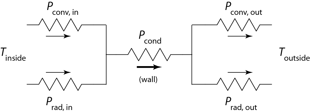
R-values for convection, radiation, and conduction combine like resistors in a circuit, shown here for a conductive wall coupling to inside and outside via convection and radiation. The sum of the two input powers equals the conducted power, which equals the sum of the output powers.
Note that when two processes operate in parallel, sharing the same area and ΔT, the effective R-value is given by Ptot = AΔT/Reff = P1 + P2 = AΔT(1/R1 + 1/R2), so that 1/Reff = (1/R1 + 1/R2). Conversely, when two processes are in series, sharing the same power flow and the same area, but piecewise-different ΔT values, we have that P = AΔT1/R1 = AΔT2/R2, so that the total ΔT = ΔT1 + ΔT2 works out to P(R1 + R2)/A, or P = AΔT/(R1 + R2), so that Reff = (R1 + R2). In other words, the R-values simply add together in series, while their inverses add when in parallel—just like resistors in an electrical circuit. Note that for the sake of tidiness I have left off the annoying 5.7 conversion factor in the above relations, which can be added back in if desired.
For an explicit example of how all this works, let’s construct a wall out of a single sheet of plywood (Κ = 0.12 W/m/°C; t = 0.019 m; so RUS = 0.9. We’ll have an inside environment with h = 2 W/m²/°C, T = 20°C, and assume the inside wall temperature is close to the same, so that I can use T = 293 K in the radiation approximation term. In this case, I compute R values (US) of 2.85 and 1 for convection and radiation, respectively (for the still air inside, radiation is here the more important channel). In parallel, these add to an effective R-value of 0.74. If the outside of our “wall” is near the ambient temperature of, say, 273 K, and a bit of wind gives us h = 10 W/m²/°C, we have R-values of 0.57 and 1.2 for convection and radiation (note the role reversal in more active air, so that convection dominates). The outside combination is R = 0.39.
Our total transfer through the wall therefore has three R-values in series: 0.74 to get heat into the wall, 0.9 to get heat through the wall, and 0.39 to get it off the outside surface. Summing these, we have RUS ˜ 2.03 in total. For an inside-outside ΔT = 20°C, each square meter of this wall would conduct 5.7×20/2.03 ˜ 56 W.
Get Real
Now that we have some sense for how to handle conduction, convection, and radiation in the R-value context, we can find and use relevant R-values for common building materials. I get most of my information from this very useful site, many values also being available at the Wikipedia site.
To compute the effective R-value for a composite surface like a wall with studs inside, one simply combines paths in parallel, weighted by the fractional area of each. For instance, a wall with studs has 15% of the area covered by studs, with a total end-to-end R-value (including convection/radiation, called “air film”) of 7.1. The other 85% is insulated bay, with an R-value of 15.7. The effective R-value is given by 1/R = (0.15/Rstud + 0.85/Rbay), calculating to R = 13.3. If I left out the insulation, I would replace the R=13 fiberglass batting with two “air film” layers carrying values of 0.68 (very similar to our value of 0.74 from above). In this case, we have 1/R = (0.15/7.1 + 0.85/4.1), or R = 4.3. Note that for uninsulated walls, the studs are more insulating than the air space between.
Let’s now assemble a table of values for relevant building blocks. Divide RUS by 5.7 to get RSI.
| Structure | % Framing | Elements | RUS |
| Uninsulated Wall | 15% | air; drywall; stud/bay; plywood; siding; air | 4.1 |
| Insulated Wall | 15% | replace bay with insulation | 13.3 |
| Uninsulated Ceiling | 8% | air; drywall; rafter/open; air | 1.65 |
| Insulated Ceiling | 8% | replace open with insulation | 13.0 |
| Uninsulated Floor | 15% | air; tile; plywood; joists/open; air | 2.5 |
| Insulated Floor | 15% | replace open with insulation | 12.7 |
| Uninsulated Roof | 8% | air; framing/open; plywood; shingles; air | 1.85 |
| Insulated Roof | 8% | replace open with insulation | 13.2 |
| Single-Pane Window | — | no coatings | 0.9 |
| Dual-Pane Window | — | half-inch air space | 2.0 |
| Best Window | — | suspended film, low E | 4.0 |
| Door | — | wood, solid core | 3.0 |
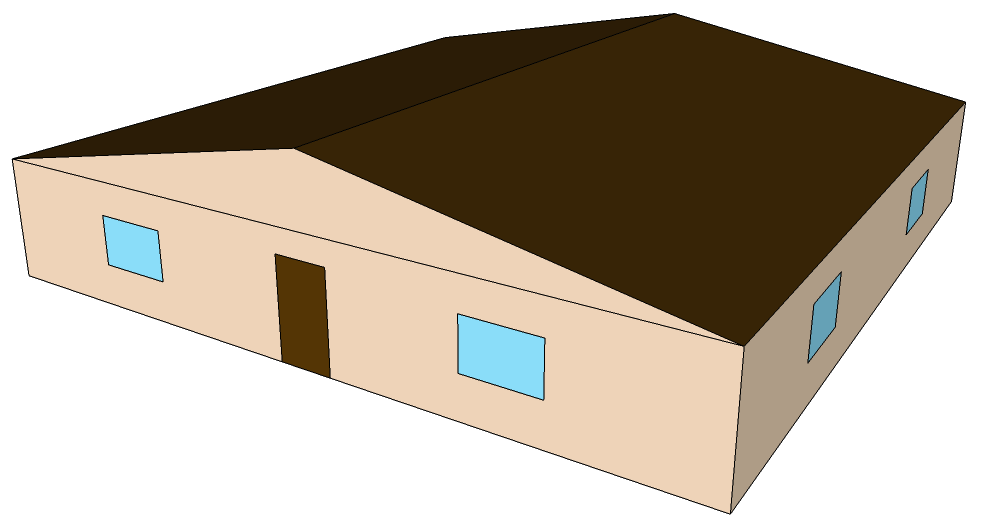
Our Boring House
For the sake of simplicity, we’re going to make a one-story house with a square footprint. We’ll have a pitched roof with attic space, and will look at raised foundations with a crawl space underneath, and also slab foundations. We’ll adorn each side of the house with two moderate-sized windows and a front and back door. For size, we’ll go with something close to the American average of 2700 ft² and take the opportunity to go metric by making our house 15 m on a side, resulting in an area of 225 m² or 2422 ft². The walls will be 2.5 m (8 ft) high. For windows, we’ll make each one 1.5 m² (equivalent to 16 ft², or 4×4 feet). Our doors will take up 2 m² each.
A beautiful house for a theorist.
The wall area therefore totals 134 m², floor and ceiling each 225 m², windows 12 m², and doors 4 m².
We will compute the thermal snugness of a house in terms of W/°C, and call this thermal admittance. Each component adds some bit of thermal admittance according to Q = P/ΔT = 5.7×A/RUS. These can then be added for each component of the house.
Using the uninsulated values for everything and single-pane windows, I get Q values, in W/°C, for the walls of 186; ceiling (assumes ample attic ventilation puts it at ambient temperature): 777; raised floor: 513; single-pane windows: 75; doors: 8. The total is 1560 W/°C.
Let’s pause to put this number in perspective. Maintaining room temperature when the outside is at freezing would require 31 kW of power, or 20 space heaters. A furnace rated at 75,000 Btu/hr is equivalent to 22 kW and would not be able to keep up. And we have not even considered drafts yet.
Now we’ll look at the other extreme and put R-13 insulation in the walls, ceiling, under the floor, and use the best windows we can buy. We will again let the attic be fully ventilated and at the outdoor ambient temperature. Now we get walls: 57; ceiling: 99; floor: 103; windows: 17, and doors still at 4. The total is 280 W/°C, and about a fifth of what it was previously. The cost of heating/cooling will likewise improve by at least a factor of five (won’t be needed as often in milder conditions). In our case, 53% of the improvement came from insulating the ceiling, 32% from the floor, 10% from the walls, and 5% from the windows. This suggests an order of priority. Of course even larger gains are possible with greater amounts of insulation—until other factors dominate.
The floor loss is slightly exaggerated here, as the simple numbers assume the crawl space is as cold as the exterior. To the degree that this is not true, the numbers soften a bit, in proportion to the relative temperature rise. It is also the case that the air near the floor is likely to be cooler than the air near the ceiling, unless the interior air is being well mixed. This also reduces heat loss through the floor in the case that it’s colder outside than inside. Still, it is likely that insulating the floor will bring a pretty noticeable improvement.
Roof Considerations
Perhaps the assumption of a fully ventilated attic caused consternation. Had I assumed a sealed attic (the other extreme), the ceiling and roof would act in series to produce an R-value of 3.5 in the uninsulated case or 26.2 in the insulated case. The thermal admittance values would then be 366 W/°C and 49 W/°C, respectively. Our totals would go from 1150 W/°C to 232 W/°C. The biggest single gain would then stem from insulating the floor. But in reality, the attic tends to be closer to ambient than to interior, so that ceiling insulation is likely to remain the most important step.
Assuming the attic is ventilated, most of the temperature difference between interior and exterior will appear across the ceiling, rendering the roof’s insulating qualities of secondary importance. But this neglects solar load onto the roof. Anyone who has experienced a hot attic knows that attic ventilation is inadequate to prevent the roof from heating the space. Therefore insulating the roof may become an important step in environments where cooling is a large energy sink. For places where heating is more important than cooling, it may actually be better to leaving the roof insulation off so that the winter sun provides some heating benefit by warming the attic a bit.
Slab Floors
For slab floors, the evaluation is somewhat more complicated than for raised floors. A six-inch slab of concrete itself has an R-value of around 0.5. But below the slab is dirt. Cobbling together information from a few sources (here and here), I gather that dry soil has a thermal conductivity around 0.8 W/m/°C, and an effective thermal thickness (length scale over which temperature gradient exists) around 0.2 m. This would give it an R-value around 1.4 for a combined slab-ground R-value of 1.9, or 2.6 once factoring in the radiative/conductive coupling. But all this may not matter because the ground temperature is pretty stable throughout the year, and may reach approximate equilibrium with your house temperature—at least away from the slab edge. To address leakage out the sides of the slab (air and ground), the Washington State site implies a loss rate of 1.2 W/°C per meter of perimeter, or 72 W/°C for our lovely house, which is not too different from what we computed for the insulated raised floor.
I Feel a Draft
Some time ago, I evaluated the thermal performance of my house (which is a slab house about two-thirds the size we’re considering in this post) in the context of heating, and in doing so computed that my house requires 610 W/°C to heat. A bit later, I looked at the cooling performance and in the process recognized a shortcoming in my previous method of analysis. A more complete method ended up suggesting 1465 W/°C. Big difference! But not only that, it seems that my house performs worse than our example house—despite being smaller, having insulation in the walls, varying degrees of insulation in the ceiling (some is very old and mashed thin), and double-pane windows virtually everywhere. In my case, the disappointing thermal performance does not translate into wasted energy, since I normally do not heat or cool the house. But a snugger house would be more comfortable. So what’s the deal?
I suspect drafts. We have ventilation fans in several rooms with minimal sealing, can lights all over the ceiling, possibly leaky door frames, and a damper in our unused fireplace that I just now checked and found open—which has probably been that way since we bought the house a few years back!
How important could drafts be? Air has a heat capacity of about 1000 J/kg/°C. Each cubic meter of air (1000 L) has about 1.25 kg of mass, and therefore holds 1250 J of energy per degree of temperature difference. Thus if air were to enter with a 10°C temperature difference at a rate of 0.1 m³/s (210 cfm, or cubic feet per minute), the corresponding thermal transport rate would be 1250 W.
Recommended flow rates call for something in excess of 4 air exchanges per hour. In our pretend house, this means 225×2.5×4 = 2250 m³ per 3600 seconds, or 0.625 m³/s, carrying about 0.8 kg/s, or 780 W/°C. That’s a lot! Another source recommends a minimum flow of 1 cfm per minute per 100 ft² of floorspace, plus another 7.5 cfm times the number of bedrooms plus one. For our model house, assuming three bedrooms, we get a minimum requirement of 54 cfm, translating to just 0.026 m³/s, or one complete exchange every six hours. Now we’re at 32 W/°C and competitive with our insulated walls, etc. I believe the latter source is more likely correct.
I found the following information from this site to be very useful:
The national average of air change rates, for existing homes, is between one and two per hour, and is dropping with tighter building practices and more stringent building codes. Standard homes built today usually have air change rates from .5 to 1.0. Extremely tight new construction can achieve air change rates of .35 or less. Most homes with such low air change rates have some form of mechanical ventilation to bring in fresh outside air and exchange heat between the two air streams.
To get an idea of what your home’s air change rate might be, consider that a tight, well sealed newly constructed home usually achieves .6 air changes per hour or less. A reasonably tight, well constructed older home typically has an air change rate of about 1 per hour. A somewhat loose older home with no storm windows and caulk missing in spots has an air change rate of about 2. A fairly loose, drafty house with no caulk or weatherstripping and entrances used might have an air change rate as high as 4, and a very drafty, dilapidated house might have an air change rate of as high as 8.
Draft Dodging
I am motivated to do a blower-door test to check the draftiness of my house. The idea is to seal up the house, install a large fan on the front door that pulls air out of the house, and measure the difference in pressure as a function of air exhaust rate. Also, once the house is under negative pressure, leaks can be hunted down by listening for whistles or hissing, using a smoke source, and partitioned by alternately closing/sealing parts of the house to isolate where the biggest problems lie. How can that not be fun?!
Another technique worth mentioning is that after tightening up a house, one can still manage to provide adequate ventilation without incurring the full thermal hit by using a heat recovery ventilator. The idea is to pass the incoming air past the outgoing air in a heat exchanger (air is separated by a thin metal membrane, for instance). By the time the air emerges from either side, the incoming air has acquired the temperature of the house’s ambient air, while the exhaust air becomes much like the exterior air before emerging. The thermal losses associated with air exchange can be cut by a factor of four or more using such an approach. This would bring the previously calculated 32 W/°C down to well less than 10, and into the same ballpark as high-performance windows.
Lessons Learned
The thermal performance of a house is not that hard to understand, given a bit of background and some relevant numbers. The tools developed here allow exploration of the relative merits of new windows, insulation projects, ventilation management, etc. Of primary importance is the ability to lump all three thermal pathways into an R-value framework so that composite structures may be evaluated and compared. By adopting units of W/°C, we can quickly understand the heating requirements for a given temperature difference, or simply use the number as an indication of thermal quality.
I encourage you to try computing the thermal admittance of your house, given its geometry and construction. If you know how many kWh or Therms per day you use to maintain a particular ΔT, you can compare the theoretical performance to measured reality.
Of course things are never as simple in practice as they are on Theoretical Lane. My house, for instance appears to be three times worse than the value I compute in ignorance of ventilation. Airflow is the wildcard here, and may indeed account for the discrepancy in my case—something I need to follow up.